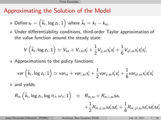
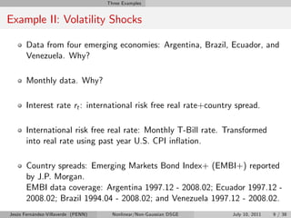
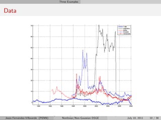
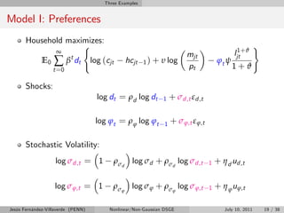
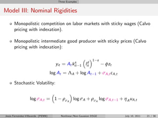
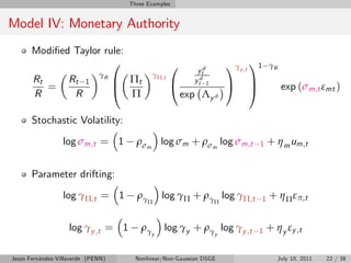
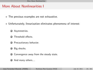
The document discusses three examples of nonlinear and non-Gaussian DSGE models. The first example features Epstein-Zin preferences to allow for a separation between risk aversion and the intertemporal elasticity of substitution. The second example models volatility shocks using time-varying variances. The third example aims to distinguish between the effects of stochastic volatility ("fortune") versus parameter drifting ("virtue") in explaining time-varying volatility in macroeconomic variables. The document outlines the motivation, structure, and solution methods for these three nonlinear DSGE models.
Saddlepoint approximations, likelihood asymptotics, and approximate condition...jaredtobin
Maximum likelihood methods may be inadequate for parameter estimation in models where many nuisance parameters are present. The modified profile likelihood (MPL) of Barndorff-Nielsen (1983) serves as a highly accurate approximation to the marginal or conditional likelihood, when either exist, and can be viewed as an approximate conditional likelihood when they do not. We examine the modified profile likelihood, its variants, and its connections with Laplace and saddlepoint approximations under both theoretical and pragmatic lenses.
AACIMP 2010 Summer School lecture by Gerhard Wilhelm Weber. "Applied Mathematics" stream. "Modern Operational Research and Its Mathematical Methods with a Focus on Financial Mathematics" course. Part 14.
More info at http://summerschool.ssa.org.ua
Aristidis Likas, Associate Professor and Christoforos Nikou, Assistant Professor, University of Ioannina, Department of Computer Science , Mixture Models for Image Analysis
Lesson 15: Exponential Growth and Decay (handout)Matthew Leingang
Many problems in nature are expressible in terms of a certain differential equation that has a solution in terms of exponential functions. We look at the equation in general and some fun applications, including radioactivity, cooling, and interest.
New Mathematical Tools for the Financial SectorSSA KPI
AACIMP 2010 Summer School lecture by Gerhard Wilhelm Weber. "Applied Mathematics" stream. "Modern Operational Research and Its Mathematical Methods with a Focus on Financial Mathematics" course. Part 5.
More info at http://summerschool.ssa.org.ua
My talk entitled "Numerical Smoothing and Hierarchical Approximations for Efficient Option Pricing and Density Estimation", that I gave at the "International Conference on Computational Finance (ICCF)", Wuppertal June 6-10, 2022. The talk is related to our recent works "Numerical Smoothing with Hierarchical Adaptive Sparse Grids and Quasi-Monte Carlo Methods for Efficient Option Pricing" (link: https://arxiv.org/abs/2111.01874) and "Multilevel Monte Carlo combined with numerical smoothing for robust and efficient option pricing and density estimation" (link: https://arxiv.org/abs/2003.05708). In these two works, we introduce the numerical smoothing technique that improves the regularity of observables when approximating expectations (or the related integration problems). We provide a smoothness analysis and we show how this technique leads to better performance for the different methods that we used (i) adaptive sparse grids, (ii) Quasi-Monte Carlo, and (iii) multilevel Monte Carlo. Our applications are option pricing and density estimation. Our approach is generic and can be applied to solve a broad class of problems, particularly for approximating distribution functions, financial Greeks computation, and risk estimation.
Option Pricing under non constant volatilityEcon 643 Fina.docxjacksnathalie
Option Pricing under non constant volatility
Econ 643: Financial Economics II
Econ 643: Financial Economics II Non constant volatility 1 / 21
Department of Economics
Introduction
Attempts have been made to fix option pricing puzzles: How to be
consistent with volatility smile and smirk.
The Gram-Charlier expansion is one of then but volatility is constant
which is inconsistent with asset return’s dynamics
We review thre approaches that aim at integrating information
embedded in past returns:
GARCH type of approach,
Stochastic volatility models: Hull and White (1987),
Stochastic volatility models: Heston (1993),
Econ 643: Financial Economics II Non constant volatility 2 / 21
The GARCH option pricing
Let St be the asset price at time t and rt = ln(St/St−1) be the log-return
process. Assume that the process rt is a (G)GARCH(1,1) process:
rt = ln
(
St
St−1
)
= µt−1 + σt−1zt, zt ∼ NID(0, 1)
σ2t = ω + α(σt−1zt − θσt−1)2 + βσ2t−1.
(1)
In this model,
µt−1 = E(rt|Jt−1) is a known function of past returns.
Ex: µt = 0, µt = µ = cst, µt = µ + λσt, µt = r + λσt − 12σ
2
t , etc.
σ2t−1 = Var(rt|Jt−1) is the conditional variance of rt given the
information Jt−1 available at t − 1.
Econ 643: Financial Economics II Non constant volatility 3 / 21
GARCH: How to price options on S?
We can rely on the risk-neutral approach:
C = e−rτ E∗ (max(ST − X, 0)) ,
where E∗ is the expectation under risk-neutral dynamics.
What is the risk-neutral dynamics of St if ln(St/St−1) is a
GARCH(1,1)?
Under risk-neutral dyn., E∗
(
St
St−1
)
= er and Var∗(rt|Jt−1) = σ2t−1
(same as under historical measure). Hence, if rt ∼ GARCH(1, 1)
under risk-neutral, the corresponding mean has to be
µ∗t−1 = r −
σ2
t−1
2
. That is:
rt = r −
σ2
t−1
2
+ σt−1z
∗
t , z
∗
t ∼ NID(0, 1)
σ2t = ω + α(σt−1z
∗
t + r −
σ2
t−1
2
− µt−1 − θσt−1)2 + βσ2t−1.
(2)
Econ 643: Financial Economics II Non constant volatility 4 / 21
GARCH: Simulating the option price
To obtain the price C by simulation:
Simulate B paths of stock price using the risk-neutral dynamics (2):
(S
(b)
t+1, S
(b)
t+2, . . . , S
(b)
T
) for b = 1, . . . , B (e.g. B = 5000).
Obtain the simulated price as
Ĉ = e−rτ Ê(max(ST − X, 0)),
with
Ê(max(ST − X, 0)) =
1
B
B
∑
b=1
max(S
(b)
T
− X, 0).
Econ 643: Financial Economics II Non constant volatility 5 / 21
Option pricing under stochastic volatility
GARCH option pricing is convenient but evidence are out that
volatility is more likely stochastic.
Option pricing under SV is quite challenging because of the extra
source of uncertainty brought by the volatility equation.
The induced PDE (by SV) for option pricing can be derived but is
hard to solve.
The most common SV option pricing models are from Hull and White
(1987) and Heston (1993).
Econ 643: Financial Economics II Non constant volatility 6 / 21
Hull and White (1987)
Consider the price process St and its instantaneous variance process
V − t = σ2t obeying the dynamics:
dS.
When trading incurs proportional costs, leverage can scale an asset's return only up to a maximum multiple, which is sensitive to the asset's volatility and liquidity. In a continuous-time model with one safe and one risky asset with constant investment opportunities and proportional transaction costs, we find the efficient portfolios that maximize long term expected returns for given average volatility. As leverage and volatility increase, rising rebalancing costs imply a declining Sharpe ratio. Beyond a critical level, even the expected return declines. For funds that seek to replicate multiples of index returns, such as leveraged ETFs, our efficient portfolios optimally trade off alpha against tracking error.
Estimation of the Latent Signals for Consensus Across Multiple Ranked Lists u...Luca Vitale
Presentation at 10th International Workshop on Simulation and Statistics. A novel method for the estimation of the underlying signal of multiple ranked lists.
Innovations in technology has revolutionized financial services to an extent that large financial institutions like Goldman Sachs are claiming to be technology companies! It is no secret that technological innovations like Data science and AI are changing fundamentally how financial products are created, tested and delivered. While it is exciting to learn about technologies themselves, there is very little guidance available to companies and financial professionals should retool and gear themselves towards the upcoming revolution.
In this master class, we will discuss key innovations in Data Science and AI and connect applications of these novel fields in forecasting and optimization. Through case studies and examples, we will demonstrate why now is the time you should invest to learn about the topics that will reshape the financial services industry of the future!
Topics in Econometrics
Numerical Smoothing and Hierarchical Approximations for E cient Option Pricin...Chiheb Ben Hammouda
My talk at the "Stochastic Numerics and Statistical Learning: Theory and Applications" Workshop at KAUST (King Abdullah University of Science and Technology), May 23, 2022, about my recent works "Numerical Smoothing with Hierarchical Adaptive Sparse Grids and Quasi-Monte Carlo Methods for Efficient Option Pricing" and "Multilevel Monte Carlo combined with numerical smoothing for robust and efficient option pricing and density estimation".
Leveraged and inverse ETFs seek a daily return equal to a multiple of an index' return, an objective that requires continuous portfolio rebalancing. The resulting trading costs create a tradeoff between tracking error, which controls the short-term correlation with the index, and excess return (or tracking difference) -- the long-term deviation from the levered index' performance. With proportional trading costs, the optimal replication policy is robust to the index' dynamics. A summary of a fund's performance is the \emph{implied spread}, equal to the product of tracking error and excess return, rescaled for leverage and average volatility. The implies spread is insensitive to the benchmark's risk premium, and offers a tool to compare the performance of funds on the same benchmark, but with different multiples and tracking errors.
Computational Tools and Techniques for Numerical Macro-Financial ModelingVictor Zhorin
A set of numerical tools used to create and analyze non-linear macroeconomic models with financial sector is discussed. New methods and results for computing Hansen-Scheinkman-Borovicka shock-price and shock-exposure elasticities for variety of models are presented. Spectral approximation technology (chebfun):
numerical computation in Chebyshev functions piece-wise smooth functions
breakpoints detection
rootfinding
functions with singularities
fast adaptive quadratures continuous QR, SVD, least-squares linear operators
solution of linear and non-linear ODE
Frechet derivatives via automatic differentiation PDEs in one space variable plus time
Stochastic processes:
(quazi) Monte-Carlo simulations, Polynomial Expansion (gPC), finite-differences (FD) non-linear IRF
Boroviˇcka-Hansen-Sc[heinkman shock-exposure and shock-price elasticities Malliavin derivatives
Many states:
Dimensionality Curse Cure
low-rank tensor decomposition
sparse Smolyak grids
Smart TV Buyer Insights Survey 2024 by 91mobiles.pdf91mobiles
91mobiles recently conducted a Smart TV Buyer Insights Survey in which we asked over 3,000 respondents about the TV they own, aspects they look at on a new TV, and their TV buying preferences.
Epistemic Interaction - tuning interfaces to provide information for AI supportAlan Dix
Paper presented at SYNERGY workshop at AVI 2024, Genoa, Italy. 3rd June 2024
https://alandix.com/academic/papers/synergy2024-epistemic/
As machine learning integrates deeper into human-computer interactions, the concept of epistemic interaction emerges, aiming to refine these interactions to enhance system adaptability. This approach encourages minor, intentional adjustments in user behaviour to enrich the data available for system learning. This paper introduces epistemic interaction within the context of human-system communication, illustrating how deliberate interaction design can improve system understanding and adaptation. Through concrete examples, we demonstrate the potential of epistemic interaction to significantly advance human-computer interaction by leveraging intuitive human communication strategies to inform system design and functionality, offering a novel pathway for enriching user-system engagements.
JMeter webinar - integration with InfluxDB and GrafanaRTTS
Watch this recorded webinar about real-time monitoring of application performance. See how to integrate Apache JMeter, the open-source leader in performance testing, with InfluxDB, the open-source time-series database, and Grafana, the open-source analytics and visualization application.
In this webinar, we will review the benefits of leveraging InfluxDB and Grafana when executing load tests and demonstrate how these tools are used to visualize performance metrics.
Length: 30 minutes
Session Overview
-------------------------------------------
During this webinar, we will cover the following topics while demonstrating the integrations of JMeter, InfluxDB and Grafana:
- What out-of-the-box solutions are available for real-time monitoring JMeter tests?
- What are the benefits of integrating InfluxDB and Grafana into the load testing stack?
- Which features are provided by Grafana?
- Demonstration of InfluxDB and Grafana using a practice web application
To view the webinar recording, go to:
https://www.rttsweb.com/jmeter-integration-webinar
Dev Dives: Train smarter, not harder – active learning and UiPath LLMs for do...UiPathCommunity
💥 Speed, accuracy, and scaling – discover the superpowers of GenAI in action with UiPath Document Understanding and Communications Mining™:
See how to accelerate model training and optimize model performance with active learning
Learn about the latest enhancements to out-of-the-box document processing – with little to no training required
Get an exclusive demo of the new family of UiPath LLMs – GenAI models specialized for processing different types of documents and messages
This is a hands-on session specifically designed for automation developers and AI enthusiasts seeking to enhance their knowledge in leveraging the latest intelligent document processing capabilities offered by UiPath.
Speakers:
👨🏫 Andras Palfi, Senior Product Manager, UiPath
👩🏫 Lenka Dulovicova, Product Program Manager, UiPath
"Impact of front-end architecture on development cost", Viktor TurskyiFwdays
I have heard many times that architecture is not important for the front-end. Also, many times I have seen how developers implement features on the front-end just following the standard rules for a framework and think that this is enough to successfully launch the project, and then the project fails. How to prevent this and what approach to choose? I have launched dozens of complex projects and during the talk we will analyze which approaches have worked for me and which have not.
Slack (or Teams) Automation for Bonterra Impact Management (fka Social Soluti...Jeffrey Haguewood
Sidekick Solutions uses Bonterra Impact Management (fka Social Solutions Apricot) and automation solutions to integrate data for business workflows.
We believe integration and automation are essential to user experience and the promise of efficient work through technology. Automation is the critical ingredient to realizing that full vision. We develop integration products and services for Bonterra Case Management software to support the deployment of automations for a variety of use cases.
This video focuses on the notifications, alerts, and approval requests using Slack for Bonterra Impact Management. The solutions covered in this webinar can also be deployed for Microsoft Teams.
Interested in deploying notification automations for Bonterra Impact Management? Contact us at sales@sidekicksolutionsllc.com to discuss next steps.
UiPath Test Automation using UiPath Test Suite series, part 3DianaGray10
Welcome to UiPath Test Automation using UiPath Test Suite series part 3. In this session, we will cover desktop automation along with UI automation.
Topics covered:
UI automation Introduction,
UI automation Sample
Desktop automation flow
Pradeep Chinnala, Senior Consultant Automation Developer @WonderBotz and UiPath MVP
Deepak Rai, Automation Practice Lead, Boundaryless Group and UiPath MVP
LF Energy Webinar: Electrical Grid Modelling and Simulation Through PowSyBl -...DanBrown980551
Do you want to learn how to model and simulate an electrical network from scratch in under an hour?
Then welcome to this PowSyBl workshop, hosted by Rte, the French Transmission System Operator (TSO)!
During the webinar, you will discover the PowSyBl ecosystem as well as handle and study an electrical network through an interactive Python notebook.
PowSyBl is an open source project hosted by LF Energy, which offers a comprehensive set of features for electrical grid modelling and simulation. Among other advanced features, PowSyBl provides:
- A fully editable and extendable library for grid component modelling;
- Visualization tools to display your network;
- Grid simulation tools, such as power flows, security analyses (with or without remedial actions) and sensitivity analyses;
The framework is mostly written in Java, with a Python binding so that Python developers can access PowSyBl functionalities as well.
What you will learn during the webinar:
- For beginners: discover PowSyBl's functionalities through a quick general presentation and the notebook, without needing any expert coding skills;
- For advanced developers: master the skills to efficiently apply PowSyBl functionalities to your real-world scenarios.
Connector Corner: Automate dynamic content and events by pushing a buttonDianaGray10
Here is something new! In our next Connector Corner webinar, we will demonstrate how you can use a single workflow to:
Create a campaign using Mailchimp with merge tags/fields
Send an interactive Slack channel message (using buttons)
Have the message received by managers and peers along with a test email for review
But there’s more:
In a second workflow supporting the same use case, you’ll see:
Your campaign sent to target colleagues for approval
If the “Approve” button is clicked, a Jira/Zendesk ticket is created for the marketing design team
But—if the “Reject” button is pushed, colleagues will be alerted via Slack message
Join us to learn more about this new, human-in-the-loop capability, brought to you by Integration Service connectors.
And...
Speakers:
Akshay Agnihotri, Product Manager
Charlie Greenberg, Host
UiPath Test Automation using UiPath Test Suite series, part 4DianaGray10
Welcome to UiPath Test Automation using UiPath Test Suite series part 4. In this session, we will cover Test Manager overview along with SAP heatmap.
The UiPath Test Manager overview with SAP heatmap webinar offers a concise yet comprehensive exploration of the role of a Test Manager within SAP environments, coupled with the utilization of heatmaps for effective testing strategies.
Participants will gain insights into the responsibilities, challenges, and best practices associated with test management in SAP projects. Additionally, the webinar delves into the significance of heatmaps as a visual aid for identifying testing priorities, areas of risk, and resource allocation within SAP landscapes. Through this session, attendees can expect to enhance their understanding of test management principles while learning practical approaches to optimize testing processes in SAP environments using heatmap visualization techniques
What will you get from this session?
1. Insights into SAP testing best practices
2. Heatmap utilization for testing
3. Optimization of testing processes
4. Demo
Topics covered:
Execution from the test manager
Orchestrator execution result
Defect reporting
SAP heatmap example with demo
Speaker:
Deepak Rai, Automation Practice Lead, Boundaryless Group and UiPath MVP
UiPath Test Automation using UiPath Test Suite series, part 4
Chapter 1 nonlinear
1. Why Nonlinear/Non-Gaussian DSGE Models?
Jesús Fernández-Villaverde
University of Pennsylvania
July 10, 2011
Jesús Fernández-Villaverde (PENN) Nonlinear/Non-Gaussian DSGE July 10, 2011 1 / 38
2. Introduction
Motivation
These lectures review recent advances in nonlinear and non-gaussian
macro model-building.
First, we will justify why we are interested in this class of models.
Then, we will study both the solution and estimation of those models.
We will work with discrete time models.
We will focus on DSGE models.
Jesús Fernández-Villaverde (PENN) Nonlinear/Non-Gaussian DSGE July 10, 2011 2 / 38
3. Introduction
Nonlinearities
Most DSGE models are nonlinear.
Common practice (you saw it yesterday): solve and estimate a
linearized version with Gaussian shocks.
Why? Stochastic neoclassical growth model is nearly linear for the
benchmark calibration (Aruoba, Fernández-Villaverde, Rubio-Ramírez,
2005).
However, we want to depart from this basic framework.
I will present three examples.
Jesús Fernández-Villaverde (PENN) Nonlinear/Non-Gaussian DSGE July 10, 2011 3 / 38
4. Three Examples
Example I: Epstein-Zin Preferences
Recursive preferences (Kreps-Porteus-Epstein-Zin-Weil) have become
a popular way to account for asset pricing observations.
Natural separation between IES and risk aversion.
Example of a more general set of preferences in macroeconomics.
Consequences for business cycles, welfare, and optimal policy design.
Link with robust control.
I study a version of the RBC with in‡ation and adjustment costs in
The Term Structure of Interest Rates in a DSGE Model with
Recursive Preferences.
Jesús Fernández-Villaverde (PENN) Nonlinear/Non-Gaussian DSGE July 10, 2011 4 / 38
6. Three Examples
Technology
Production function:
yt = kt (zt lt )1
ζ ζ
Law of motion:
log zt +1 = λ log zt + χσε εzt +1 where εzt N (0, 1)
Aggregate constraints:
ct + it = kt (zt lt )1
ζ ζ
kt +1 = (1 δ) kt + it
Jesús Fernández-Villaverde (PENN) Nonlinear/Non-Gaussian DSGE July 10, 2011 6 / 38
7. Three Examples
Approximating the Solution of the Model
b b
De…ne st = kt , log zt ; 1 where kt = kt kss .
Under di¤erentiability conditions, third-order Taylor approximation of
the value function around the steady state:
1 1
V kt , log zt ; 1 ' Vss + Vi ,ss sti + Vij ,ss sti stj + Vijl ,ss sti stj stl ,
b
2 6
Approximations to the policy functions:
1 1
var kt , log zt ; 1 ' varss + vari ,ss sti + varij ,ss sti stj + varijl ,ss sti stj stl
b
2 6
and yields:
b
Rm kt , log zt , log π t , ω t ; 1 ' Rm,ss + Rm,i ,ss sat
1 i j 1 i j l
+ Rm,ij ,ss sat sat + Rm,ijl ,ss sat sat sat
2 6
Jesús Fernández-Villaverde (PENN) Nonlinear/Non-Gaussian DSGE July 10, 2011 7 / 38
8. Three Examples
Structure of Approximation
1 The constant terms Vss , varss , or Rm,ss do not depend on γ, the
parameter that controls risk aversion.
2 None of the terms in the …rst-order approximation, V.,ss , var.,ss , or
Rm,.,ss (for all m) depend on γ.
3 None of the terms in the second-order approximation, V..,ss , var..,ss ,
or Rm,..,ss depend on γ, except V33,ss , var33,ss , and Rm,33,ss (for all
m). This last term is a constant that captures precautionary behavior.
4 In the third-order approximation only the terms of the form V33.,ss ,
V3.3,ss , V.33,ss and var33.,ss , var3.3,ss , var.33,ss and Rm,33.,ss , Rm,3.3,ss ,
Rm,.33,ss (for all m) that is, terms on functions of χ2 , depend on γ.
Jesús Fernández-Villaverde (PENN) Nonlinear/Non-Gaussian DSGE July 10, 2011 8 / 38
9. Three Examples
Example II: Volatility Shocks
Data from four emerging economies: Argentina, Brazil, Ecuador, and
Venezuela. Why?
Monthly data. Why?
Interest rate rt : international risk free real rate+country spread.
International risk free real rate: Monthly T-Bill rate. Transformed
into real rate using past year U.S. CPI in‡ation.
Country spreads: Emerging Markets Bond Index+ (EMBI+) reported
by J.P. Morgan.
EMBI data coverage: Argentina 1997.12 - 2008.02; Ecuador 1997.12 -
2008.02; Brazil 1994.04 - 2008.02; and Venezuela 1997.12 - 2008.02.
Jesús Fernández-Villaverde (PENN) Nonlinear/Non-Gaussian DSGE July 10, 2011 9 / 38
10. Three Examples
Data
Figure: Country Spreads and DSGE Real Rate
Jesús Fernández-Villaverde (PENN) Nonlinear/Non-Gaussian T-Bill July 10, 2011 10 / 38
11. Three Examples
The Law of Motion for Interest Rates
Decomposition of interest rates:
rt = |{z} +
r εtb,t + εr ,t
|{z} |{z}
mean T-Bill shocks Spread shocks
εtb,t and εr ,t follow:
εtb,t = ρtb εtb,t 1 + e σtb,t utb,t , utb,t N (0, 1)
εr ,t = ρr εr ,t 1 + e σr ,t ur ,t , ur ,t N (0, 1)
σtb,t and σr ,t follow:
σtb,t = 1 ρσtb σtb + ρσtb σtb,t 1 + η tb uσtb ,t , uσtb ,t N (0, 1)
σr ,t = 1 ρσr σr + ρσr σr ,t 1 + η r uσr ,t , uσr ,t N (0, 1)
I could also allow for correlations of shocks.
Jesús Fernández-Villaverde (PENN) Nonlinear/Non-Gaussian DSGE July 10, 2011 11 / 38
12. Three Examples
A Small Open Economy Model I
Risk Matters: The Real E¤ects of Volatility Shocks.
Prototypical small open economy model: Mendoza (1991), Correia et
al. (1995), Neumeyer and Perri (2005), Uribe and Yue (2006).
Representative household with preferences:
∞ Ct ω 1H ω 1 v 1
∑β t t
E0 .
t =0 1 v
Why Greenwood-Hercowitz-Hu¤man (GHH) preferences? Absence of
wealth e¤ects.
Jesús Fernández-Villaverde (PENN) Nonlinear/Non-Gaussian DSGE July 10, 2011 12 / 38
13. Three Examples
A Small Open Economy Model II
Interest rates:
rt = r + εtb,t + εr ,t
εtb,t = ρtb εtb,t 1 + e σtb,t utb,t , utb,t N (0, 1)
σr ,t
εr ,t = ρr εr ,t 1 +e ur ,t , ur ,t N (0, 1)
σtb,t = 1 ρσtb σtb + ρσtb σtb,t 1 + η tb uσtb ,t , uσtb ,t N (0, 1)
σr ,t = 1 ρσr σr + ρσr σr ,t 1 + η r uσr ,t , uσr ,t N (0, 1)
Household’ budget constraint:
s
Dt + 1 Φd
= Dt Wt Ht Rt Kt + Ct + It + ( Dt + 1 D )2
1 + rt 2
Role of Φd > 0 (Schmitt-Grohé and Uribe, 2003).
Jesús Fernández-Villaverde (PENN) Nonlinear/Non-Gaussian DSGE July 10, 2011 13 / 38
14. Three Examples
A Small Open Economy Model III
The stock of capital evolves according to the following law of motion:
!
2
φ It
Kt + 1 = ( 1 δ ) Kt + 1 1 It
2 It 1
Typical no-Ponzi condition.
Production function:
1 α
Yt = Ktα e X t Ht
where:
Xt = ρx Xt 1 + e σx ux ,t , ux ,t N (0, 1) .
Competitive equilibrium de…ned in a standard way.
Jesús Fernández-Villaverde (PENN) Nonlinear/Non-Gaussian DSGE July 10, 2011 14 / 38
15. Three Examples
Solving the Model
Perturbation methods.
We are interested on the e¤ects of a volatility increase, i.e., a positive
shock to either uσr ,t or uσtb ,t , while ur ,t = 0 and utb,t = 0.
We need to obtain a third approximation of the policy functions:
1 A …rst order approximation satis…es a certainty equivalence principle.
Only level shocks utb,t , ur ,t , and uX ,t appear.
2 A second order approximation only captures volatility indirectly via
cross products ur ,t uσr ,t and utb,t uσtb ,t ,. Thus, volatility only has an
e¤ect if the real interest rate changes.
3 In the third order, volatility shocks, uσ,t and uσtb ,t , enter as
independent arguments.
Moreover:
1 Cubic terms are quantitatively important.
2 The mean of the ergodic distributions of the endogenous variables and
the deterministic steady state values are quite di¤erent. Key for
calibration.
Jesús Fernández-Villaverde (PENN) Nonlinear/Non-Gaussian DSGE July 10, 2011 15 / 38
16. Three Examples
Example III: Fortune or Virtue
Strong evidence of time-varying volatility of U.S. aggregate variables.
Most famous example: the Great Moderation between 1984 and 2007.
Two explanations:
1 Stochastic volatility: fortune.
2 Parameter drifting: virtue.
How can we measure the impact of each of these two mechanisms?
We build and estimate a medium-scale DSGE model with:
1 Stochastic volatility in the shocks that drive the economy.
2 Parameter drifting in the monetary policy rule.
Jesús Fernández-Villaverde (PENN) Nonlinear/Non-Gaussian DSGE July 10, 2011 16 / 38
17. Three Examples
The Discussion
Starting point in empirical work by Kim and Nelson (1999) and
McConnell and Pérez-Quirós (2000).
Virtue: Clarida, Galí, and Gertler (2000) and Lubik and Schorfheide
(2004).
Sims and Zha (2006): once time-varying volatility is allowed in a
SVAR model, data prefer fortune.
Follow-up papers: Canova and Gambetti (2004), Cogley and Sargent
(2005), Primiceri (2005).
Fortune papers are SVARs models: Benati and Surico (2009).
A DSGE model with both features is a natural measurement tool.
Jesús Fernández-Villaverde (PENN) Nonlinear/Non-Gaussian DSGE July 10, 2011 17 / 38
18. Three Examples
The Goals
1 How do we write a medium-scale DSGE with stochastic volatility and
parameter drifting?
2 How do we evaluate the likelihood of the model and how to
characterize the decision rules of the equilibrium?
3 How do we estimate the model using U.S. data and assess model …t?
4 How do we build counterfactual histories?
Jesús Fernández-Villaverde (PENN) Nonlinear/Non-Gaussian DSGE July 10, 2011 18 / 38
20. Three Examples
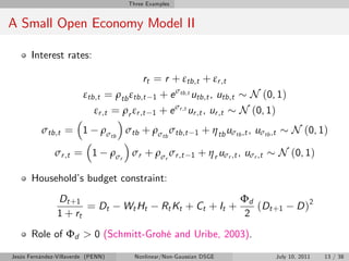
Model II: Constraints
Budget constraint:
Z
mjt bjt +1
cjt + xjt + + + qjt +1,t ajt +1 d ω j ,t +1,t =
pt pt
mjt 1 bjt
wjt ljt + rt ujt µt 1 Φ [ujt ] kjt 1 + + Rt 1 + ajt + Tt + zt
pt pt
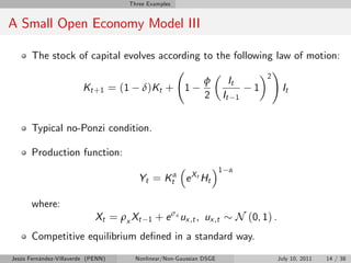
The capital evolves:
xjt
kjt = (1 δ) kjt 1 + µt 1 V xjt
xjt 1
Investment-speci…c productivity µt follows a random walk in logs:
log µt = Λµ + log µt 1 + σµ,t εµ,t
Stochastic Volatility:
log σµ,t = 1 ρσµ log σ + ρ
µ σµ log σµ,t 1 + η µ uµ,t
Jesús Fernández-Villaverde (PENN) Nonlinear/Non-Gaussian DSGE July 10, 2011 20 / 38
21. Three Examples
Model III: Nominal Rigidities
Monopolistic competition on labor markets with sticky wages (Calvo
pricing with indexation).
Monopolistic intermediate good producer with sticky prices (Calvo
pricing with indexation):
1 α
α d
yit = At kit 1 lit φzt
log At = ΛA + log At 1 + σA,t εA,t
Stochastic Volatility:
log σA,t = 1 ρσA log σA + ρσA log σA,t 1 + η A uA,t
Jesús Fernández-Villaverde (PENN) Nonlinear/Non-Gaussian DSGE July 10, 2011 21 / 38
22. Three Examples
Model IV: Monetary Authority
Modi…ed Taylor rule:
0 0 1γy ,t 11 γR
ytd
B Πt
γR γΠ,t
Rt Rt 1 @ ytd 1
A C
= @ A exp (σm,t εmt )
R R Π exp Λy d
Stochastic Volatility:
log σm,t = 1 ρσm log σm + ρσm log σm,t 1 + η m um,t
Parameter drifting:
log γΠ,t = 1 ργ log γΠ + ργ log γΠ,t 1 + η Π επ,t
Π Π
log γy ,t = 1 ργ log γy + ργ log γy ,t 1 + η y εy ,t
y y
Jesús Fernández-Villaverde (PENN) Nonlinear/Non-Gaussian DSGE July 10, 2011 22 / 38
23. More About Nonlinearities
More About Nonlinearities I
The previous examples are not exhaustive.
Unfortunately, linearization eliminates phenomena of interest:
1 Asymmetries.
2 Threshold e¤ects.
3 Precautionary behavior.
4 Big shocks.
5 Convergence away from the steady state.
6 And many others....
Jesús Fernández-Villaverde (PENN) Nonlinear/Non-Gaussian DSGE July 10, 2011 23 / 38
24. More About Nonlinearities
More About Nonlinearities II
Linearization limits our study of dynamics:
1 Zero bound on the nominal interest rate.
2 Finite escape time.
3 Multiple steady states.
4 Limit cycles.
5 Subharmonic, harmonic, or almost-periodic oscillations.
6 Chaos.
Jesús Fernández-Villaverde (PENN) Nonlinear/Non-Gaussian DSGE July 10, 2011 24 / 38
25. More About Nonlinearities
More About Nonlinearities III
Moreover, linearization induces an approximation error.
This is worse than you may think.
1 Theoretical arguments:
1 Second-order errors in the approximated policy function imply
…rst-order errors in the loglikelihood function.
2 As the sample size grows, the error in the likelihood function also grows
and we may have inconsistent point estimates.
3 Linearization complicates the identi…cation of parameters.
2 Computational evidence.
Jesús Fernández-Villaverde (PENN) Nonlinear/Non-Gaussian DSGE July 10, 2011 25 / 38
26. More About Nonlinearities
Arguments Against Nonlinearities
1 Theoretical reasons: we know way less about nonlinear and
non-gaussian systems.
2 Computational limitations.
3 Bias.
Mark Twain
To a man with a hammer, everything looks like a nail.
Teller’ Law
s
A state-of-the-art computation requires 100 hours of CPU time on the
state-of-the art computer, independent of the decade.
Jesús Fernández-Villaverde (PENN) Nonlinear/Non-Gaussian DSGE July 10, 2011 26 / 38
27. Solution
Solving DSGE Models
We want to have a general formalism to think about solving DSGE
models.
We need to move beyond value function iteration.
Theory of functional equations.
We can cast numerous problems in macroeconomics involve
functional equations.
Examples: Value Function, Euler Equations.
Jesús Fernández-Villaverde (PENN) Nonlinear/Non-Gaussian DSGE July 10, 2011 27 / 38
28. Solution
Functional Equation
Let J 1 and J 2 be two functional spaces, Ω <l and let H : J 1 ! J 2
be an operator between these two spaces.
A functional equation problem is to …nd a function d : Ω ! <m such
that
H (d ) = 0
Regular equations are particular examples of functional equations.
Note that 0 is the space zero, di¤erent in general that the zero in the
reals.
Jesús Fernández-Villaverde (PENN) Nonlinear/Non-Gaussian DSGE July 10, 2011 28 / 38
29. Solution
Example: Euler Equation I
Take the basic RBC:
∞
max E0 ∑ β t u ( ct )
t =0
ct + kt +1 = e zt ktα
+ (1 δ) kt , 8 t > 0
zt = ρzt 1 + σεt , εt N (0, 1)
The …rst order condition:
u 0 (ct ) = βEt u 0 (ct +1 ) 1 + αe zt +1 ktα+1
1
δ
There is a policy function g : <+ < ! <2 that gives the optimal
+
choice of consumption and capital tomorrow given capital and
productivity today.
Jesús Fernández-Villaverde (PENN) Nonlinear/Non-Gaussian DSGE July 10, 2011 29 / 38
30. Solution
Example: Euler Equation II
Then:
u 0 g 1 (kt , zt ) = βEt u 0 g 1 (kt +1 , zt +1 ) 1 + f g 2 (kt , zt ) , zt +1 δ
or, alternatively:
u 0 g 1 (kt , zt )
βEt u 0 g 1 g 2 (kt , zt ) , zt +1 1 + f g 2 (kt , zt ) , zt +1 δ =0
We have functional equation where the unknown object is the policy
function g ( ).
More precisely, an integral equation (expectation operator). This can
lead to some measure theoretic issues that we will ignore.
Jesús Fernández-Villaverde (PENN) Nonlinear/Non-Gaussian DSGE July 10, 2011 30 / 38
31. Solution
Example: Euler Equation III
Mapping into an operator is straightforward:
H = u0 ( ) βEt u 0 ( ) (1 + f ( , zt +1 ) δ)
d =g
If we …nd g , and a transversality condition is satis…ed, we are done!
Jesús Fernández-Villaverde (PENN) Nonlinear/Non-Gaussian DSGE July 10, 2011 31 / 38
32. Solution
Example: Euler Equation IV
Slightly di¤erent de…nitions of H and d can be used.
For instance if we take again the Euler equation:
u 0 ( ct ) βEt u 0 (ct +1 ) 1 + αe zt +1 ktα+1
1
δ =0
we may be interested in …nding the unknown conditional expectation
Et u 0 (ct +1 ) 1 + αe zt +1 ktα+1 δ .
1
Since Et is itself another function, we write
H (d ) = u 0 ( ) βd = 0
where d = Et fϑ g and ϑ = u 0 ( ) (1 + f ( , zt +1 ) δ) .
Jesús Fernández-Villaverde (PENN) Nonlinear/Non-Gaussian DSGE July 10, 2011 32 / 38
33. Solution
How Do We Solve Functional Equations?
Two Main Approaches
1 Perturbation Methods:
n
d n (x, θ ) = ∑ θ i (x x0 )i
i =0
We use implicit-function theorems to …nd coe¢ cients θ i .
2 Projection Methods:
n
d n (x, θ ) = ∑ θ i Ψi (x )
i =0
We pick a basis fΨi (x )gi∞ 0 and “project” H ( ) against that basis.
=
Jesús Fernández-Villaverde (PENN) Nonlinear/Non-Gaussian DSGE July 10, 2011 33 / 38
34. Solution
Relation with Value Function Iteration
There is a third main approach: the dynamic programing algorithm.
Advantages:
1 Strong theoretical properties.
2 Intuitive interpretation.
Problems:
1 Di¢ cult to use with non-pareto e¢ cient economies.
2 Curse of dimensionality.
Jesús Fernández-Villaverde (PENN) Nonlinear/Non-Gaussian DSGE July 10, 2011 34 / 38
35. Estimation
Evaluating the Likelihood Function
How do we take the model to the data?
Usually we cannot write the likelihood of a DSGE model.
Once the model is nonlinear and/or non-gaussian we cannot use the
Kalman …lter to evaluate the likelihood function of the model.
How do we evaluate then such likelihood? Using Sequential Monte
Carlo.
Jesús Fernández-Villaverde (PENN) Nonlinear/Non-Gaussian DSGE July 10, 2011 35 / 38
36. Estimation
Basic Estimation Algorithm 1: Evaluating Likelihood
Input: observables Y T , DSGE model M with parameters
γ 2 Υ.
Output: likelihood p y T ; γ .
1 Given γ, solve for policy functions of M.
2 With the policy functions, write the state-space form:
St = f ( St 1 , Wt ; γ i )
Yt = g (St , Vt ; γi )
3 With state space form, evaluate likelihood:
T
p y T ; γi = ∏p yt jy t 1
; γi
t =1
Jesús Fernández-Villaverde (PENN) Nonlinear/Non-Gaussian DSGE July 10, 2011 36 / 38
37. Estimation
Basic Estimation Algorithm 2: MLE
Input: observables Y T , DSGE model M parameterized by
γ 2 Υ.
Estimates: b
γ
1 Set i = 0. Fix initial parameter values γi .
2 Compute p y T ; γi using algorithm 1.
3 Is γi = arg max p y T ; γ ?
1 Yes: b
Make γ = γi . Stop.
2 No: Make γi γ i +1 . Go to step 2.
Jesús Fernández-Villaverde (PENN) Nonlinear/Non-Gaussian DSGE July 10, 2011 37 / 38
38. Estimation
Basic Estimation Algorithm 3: Bayesian
Input: observables Y T , DSGE model M parameterized by
γ 2 Υ with priors π (γ).
Posterior distribution: π γj Y T
1 Fix I . Set i = 0 and chose initial parameter values γi .
2 Compute p y T ; γi using algorithm 1.
3 Propose γ = γi + ε where ε N (0, Σ) .
p (y T ;γ )π (γ )
4 Compute α = min p (y T ;γi )π (γi )
,1 .
5 With probability α, make γi +1 = γ . Otherwise γi +1 = γi .
6 If i < M, i ı + 1.
¯ Go to step 3. Otherwise Stop.
Jesús Fernández-Villaverde (PENN) Nonlinear/Non-Gaussian DSGE July 10, 2011 38 / 38