Download to read offline
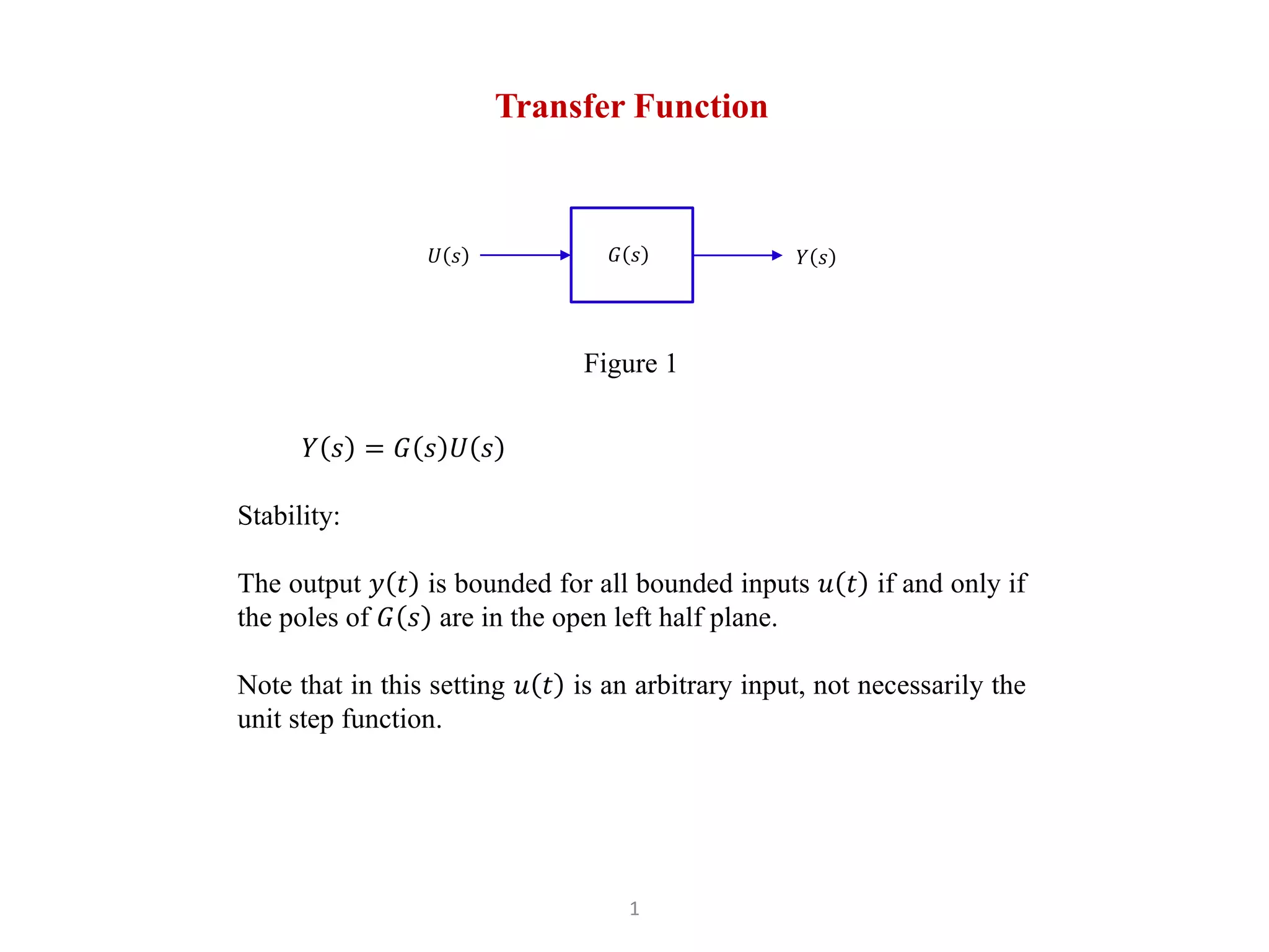
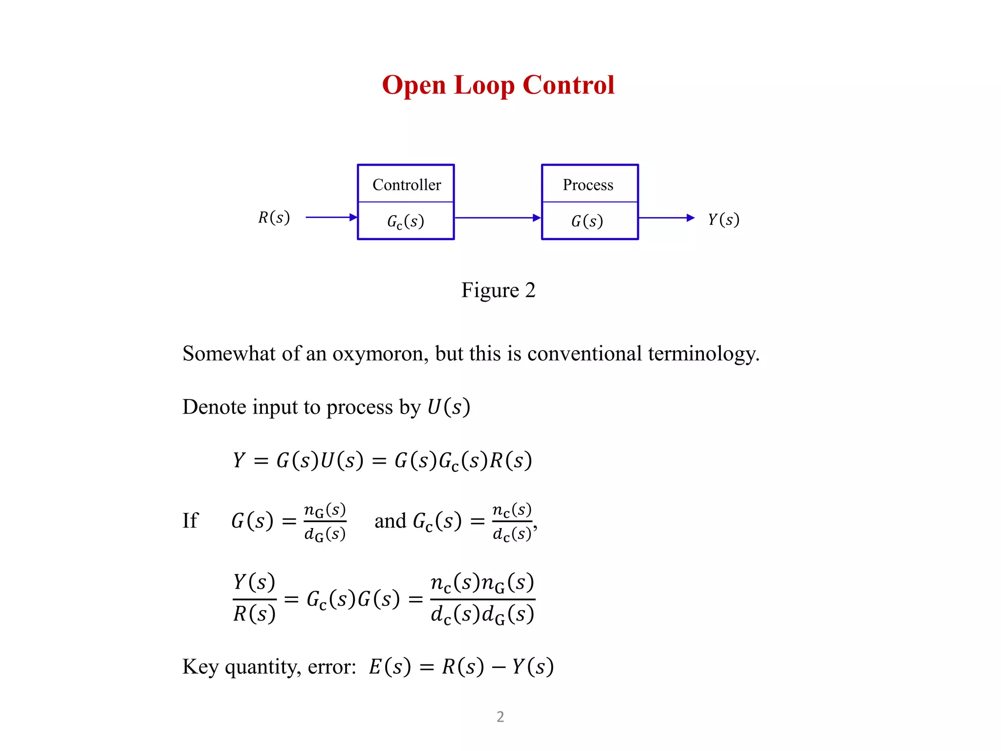
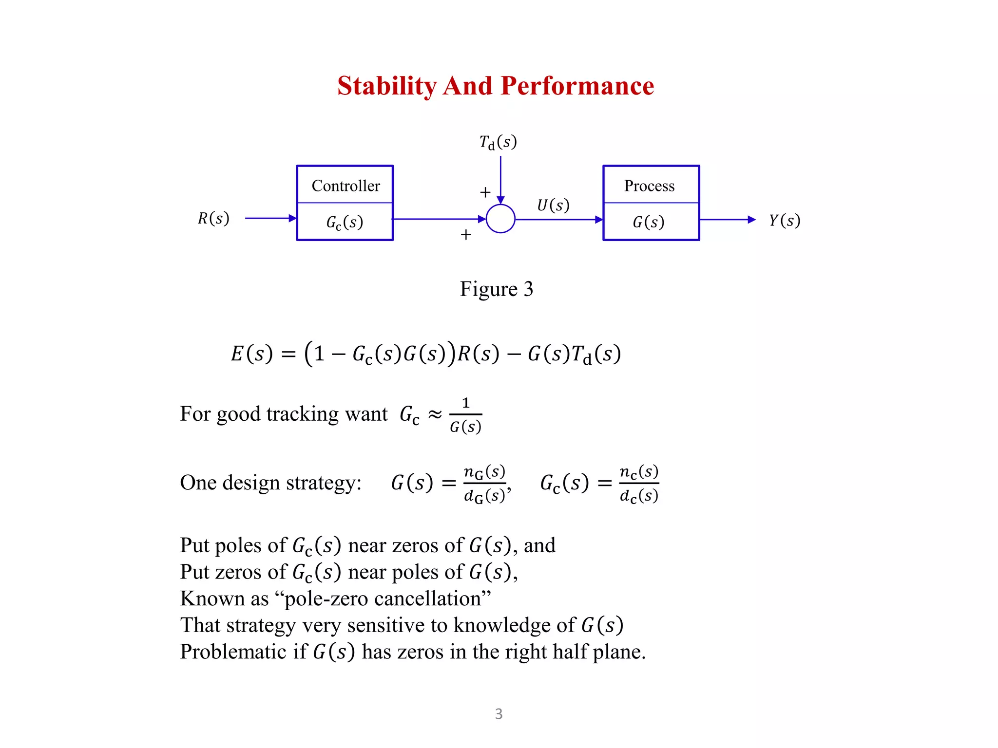
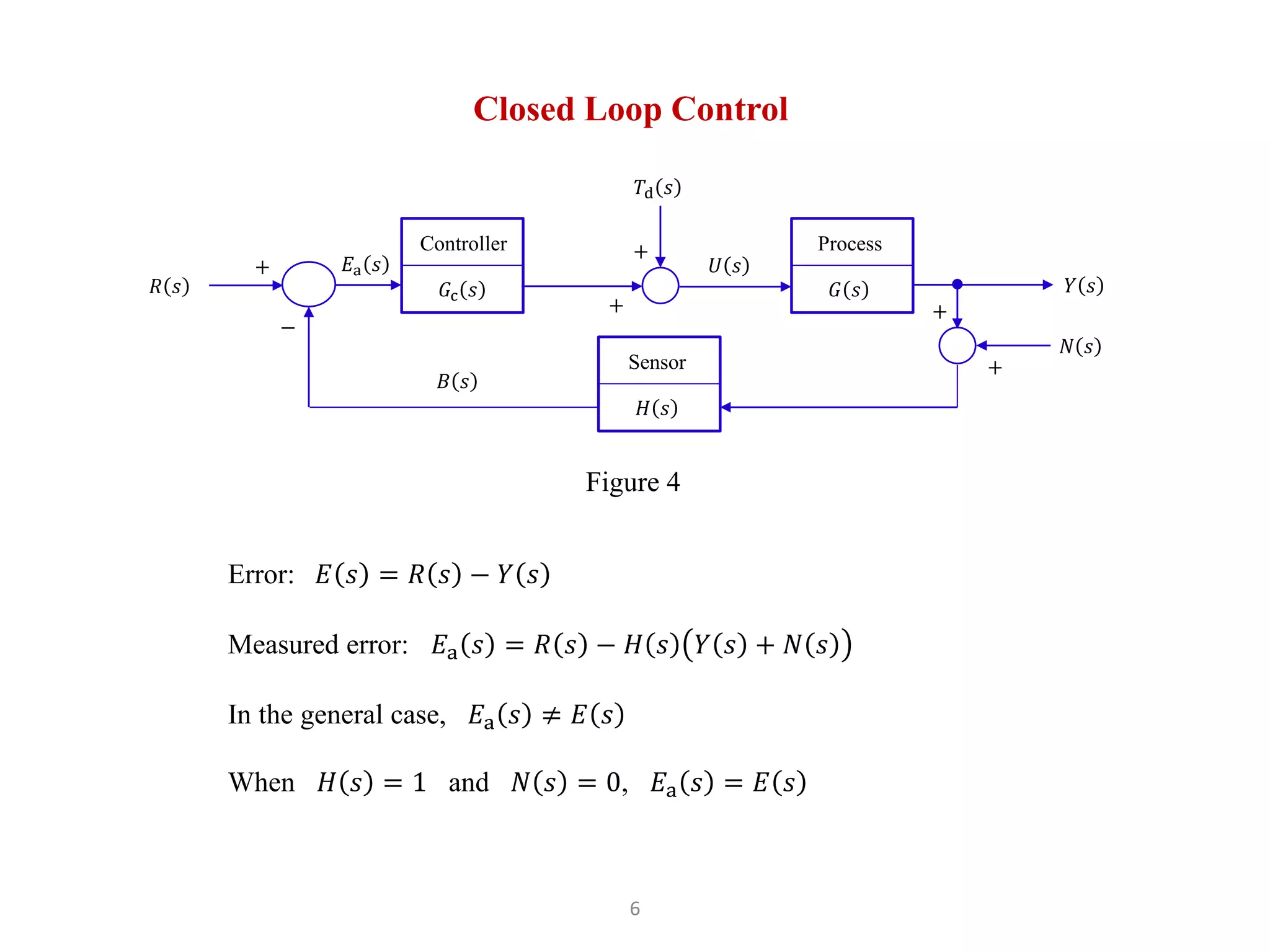
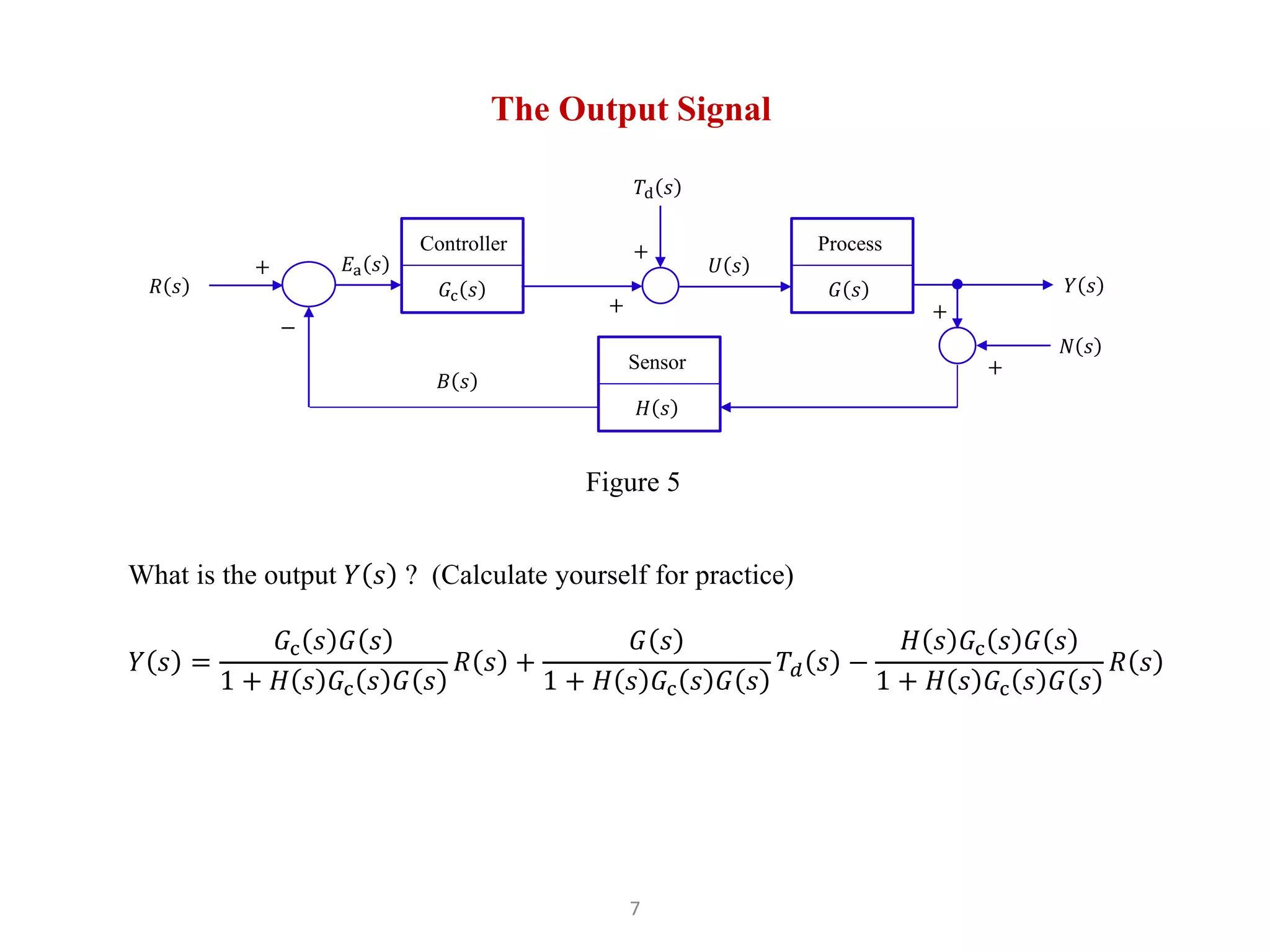
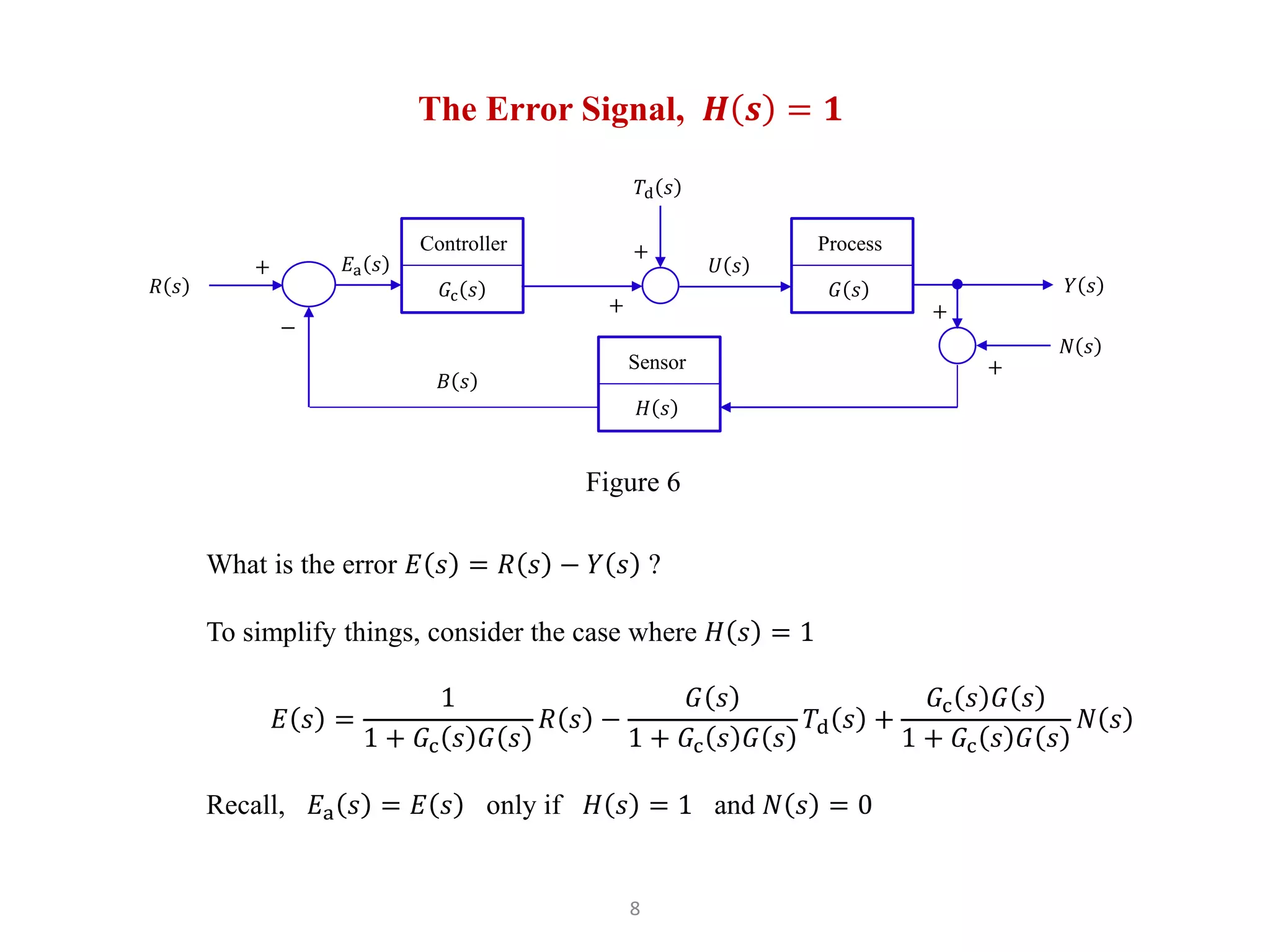
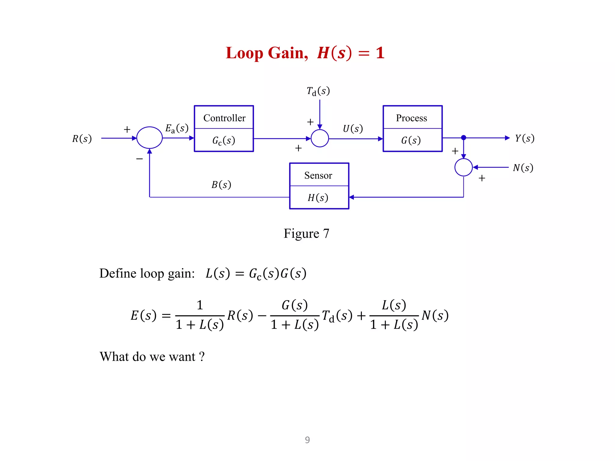
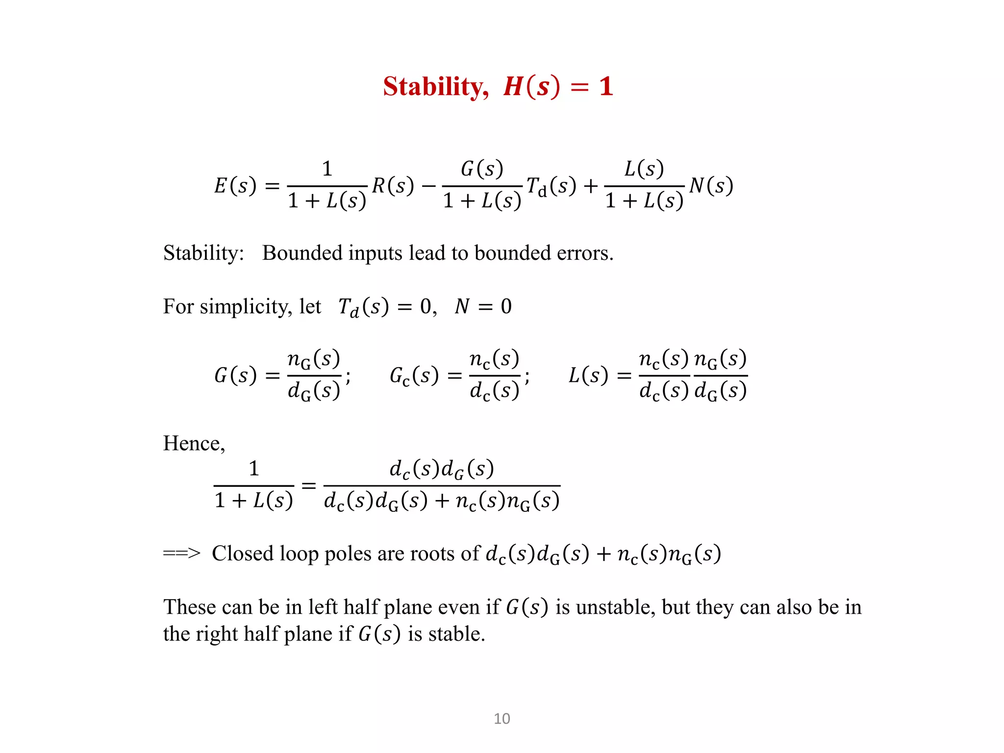
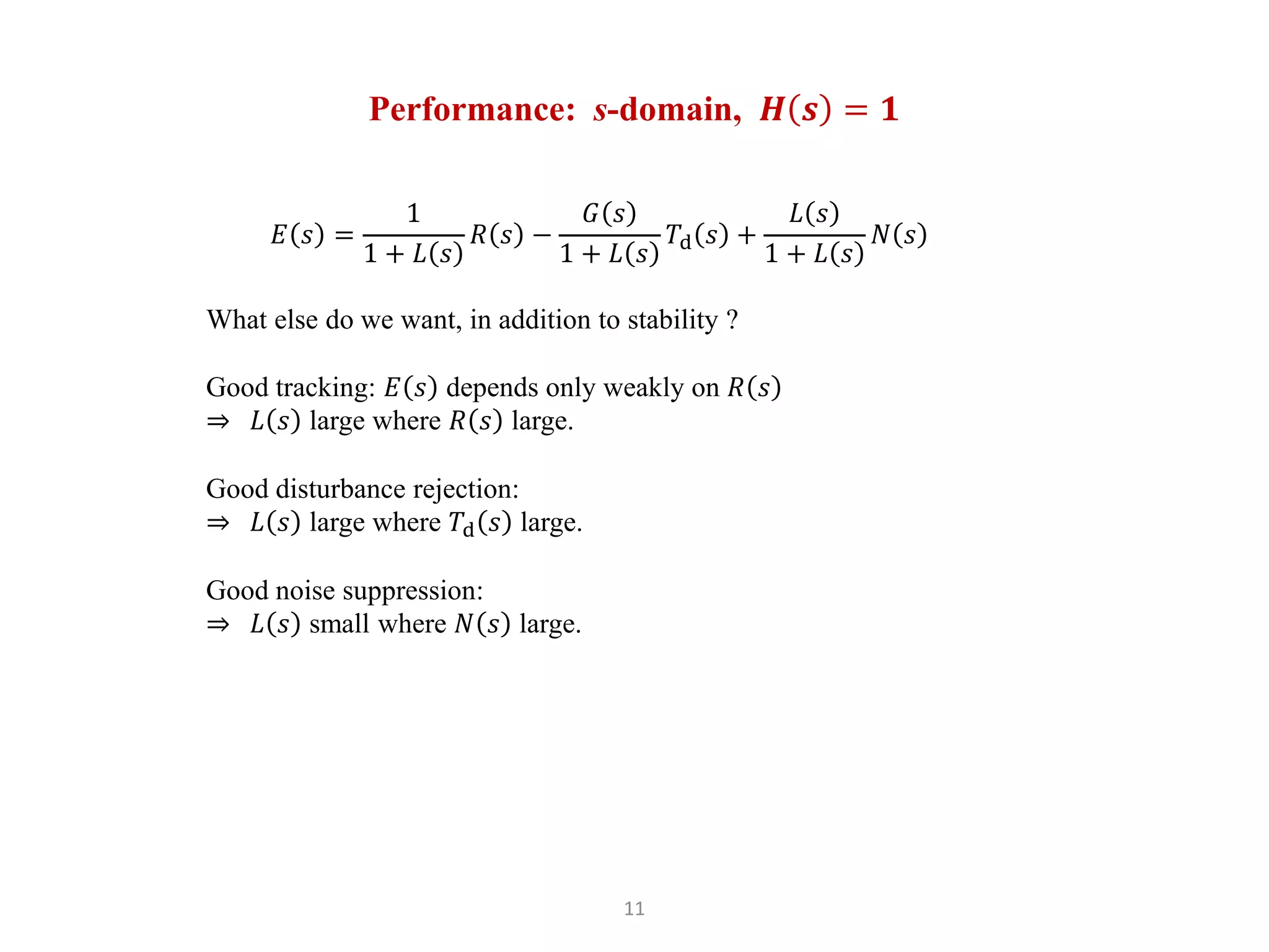
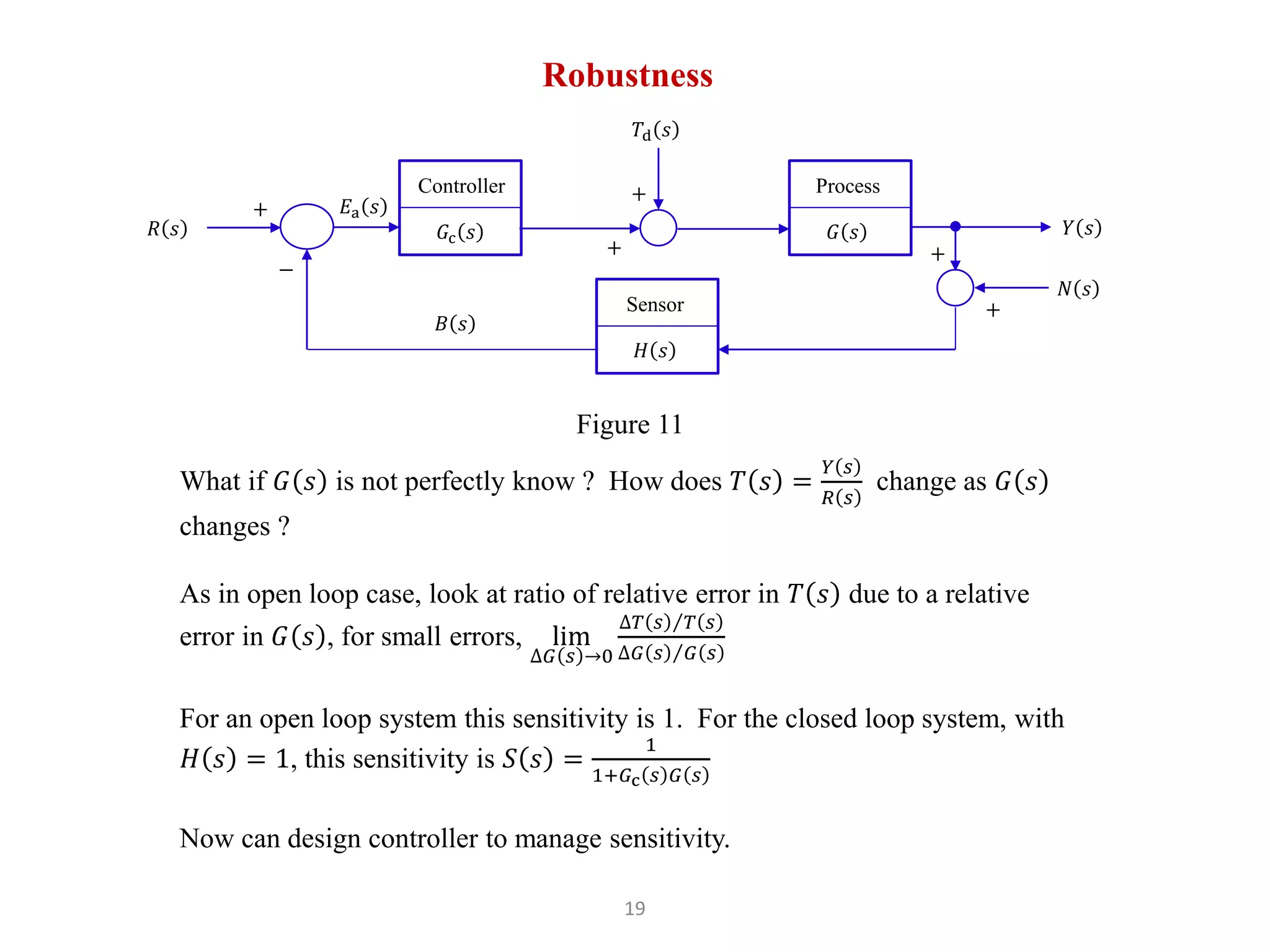
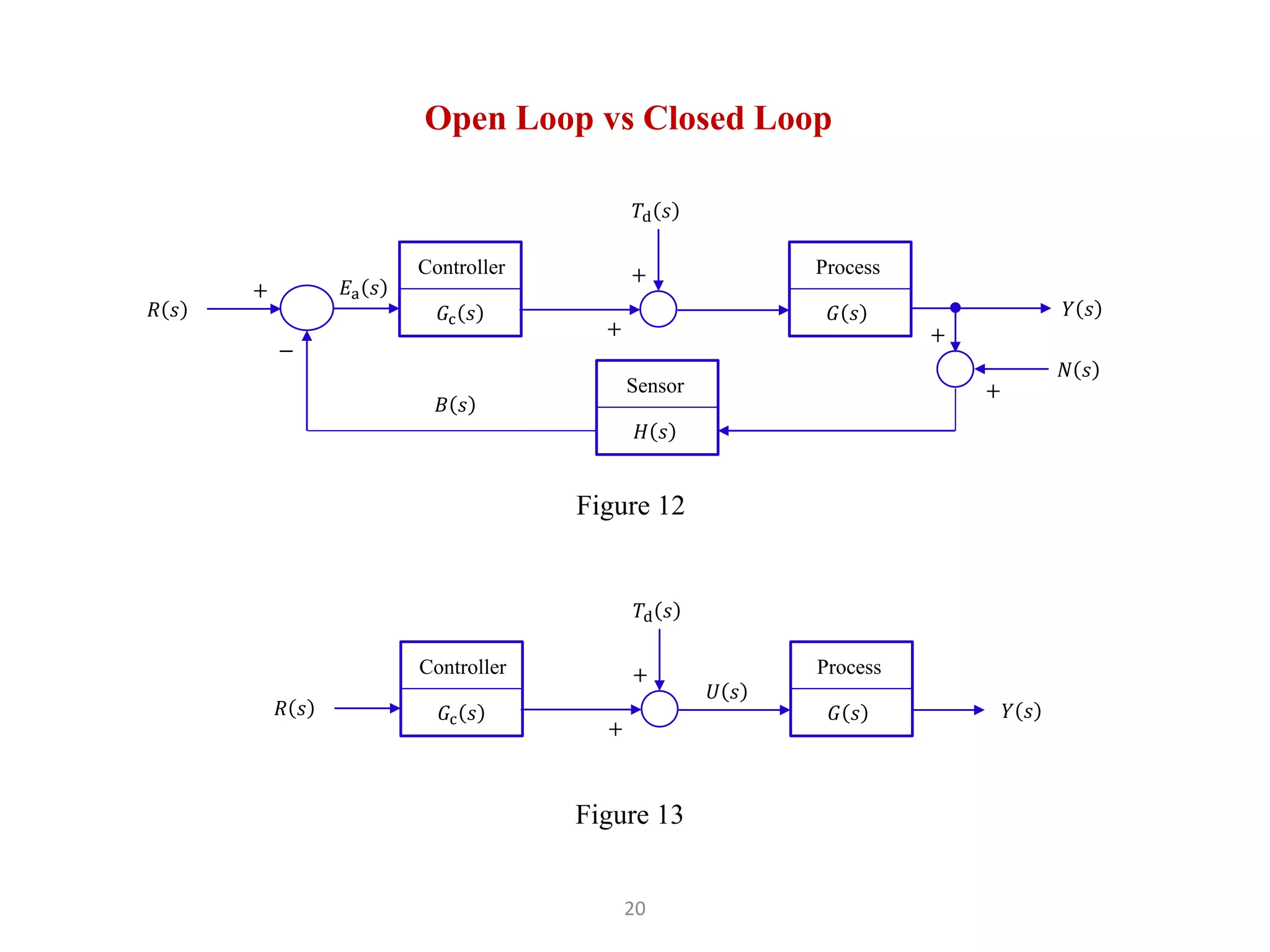
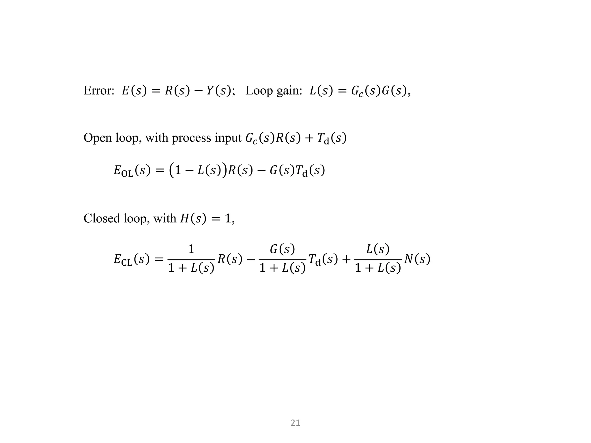
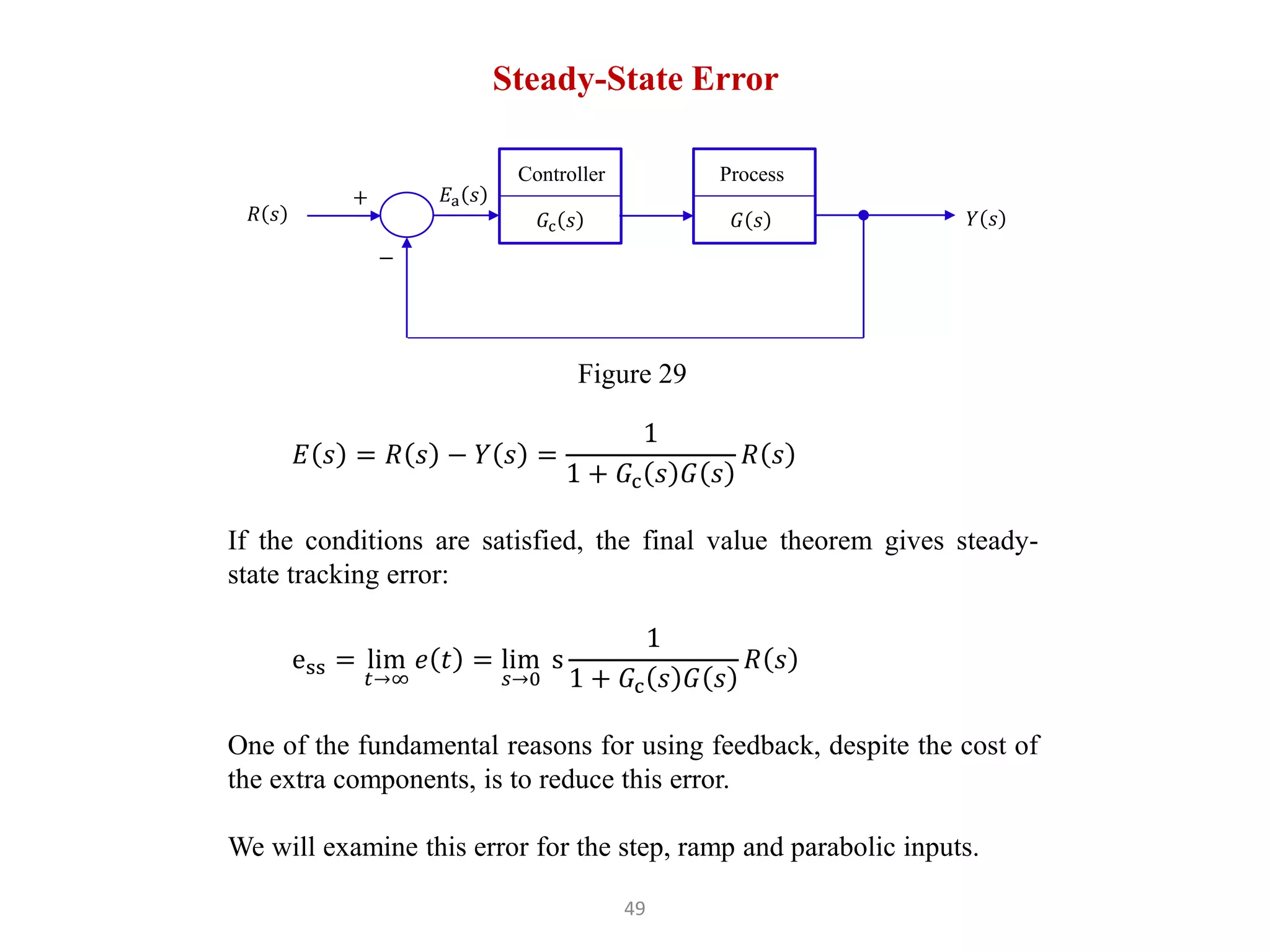
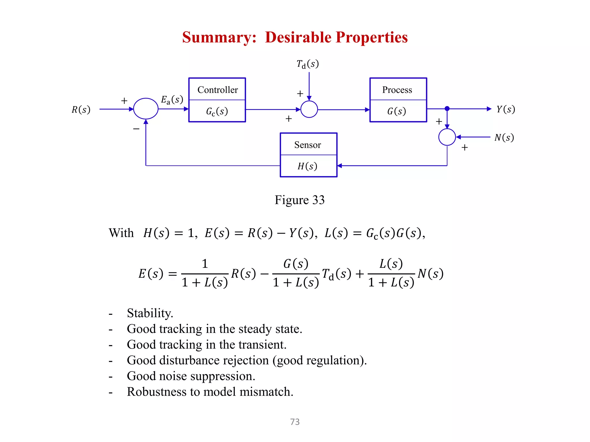

The document discusses fundamentals of feedback control systems, including: 1) Feedback control systems use a transfer function to relate the output (Y(s)) to the input (U(s)) as Y(s) = G(s)U(s), where stability requires the poles of G(s) be in the left half plane. 2) Open loop control has the error E(s) = R(s) - Y(s) where the controller Gc(s) cannot reject disturbances. 3) Closed loop control uses feedback to measure the error Ea(s) = R(s) - H(s)Y(s) + N(s) and