This document discusses various regularization techniques for deep learning models. It defines regularization as any modification to a learning algorithm intended to reduce generalization error without affecting training error. It then describes several specific regularization methods, including weight decay, norm penalties, dataset augmentation, early stopping, dropout, adversarial training, and tangent propagation. The goal of regularization is to reduce overfitting and improve generalizability of deep learning models.

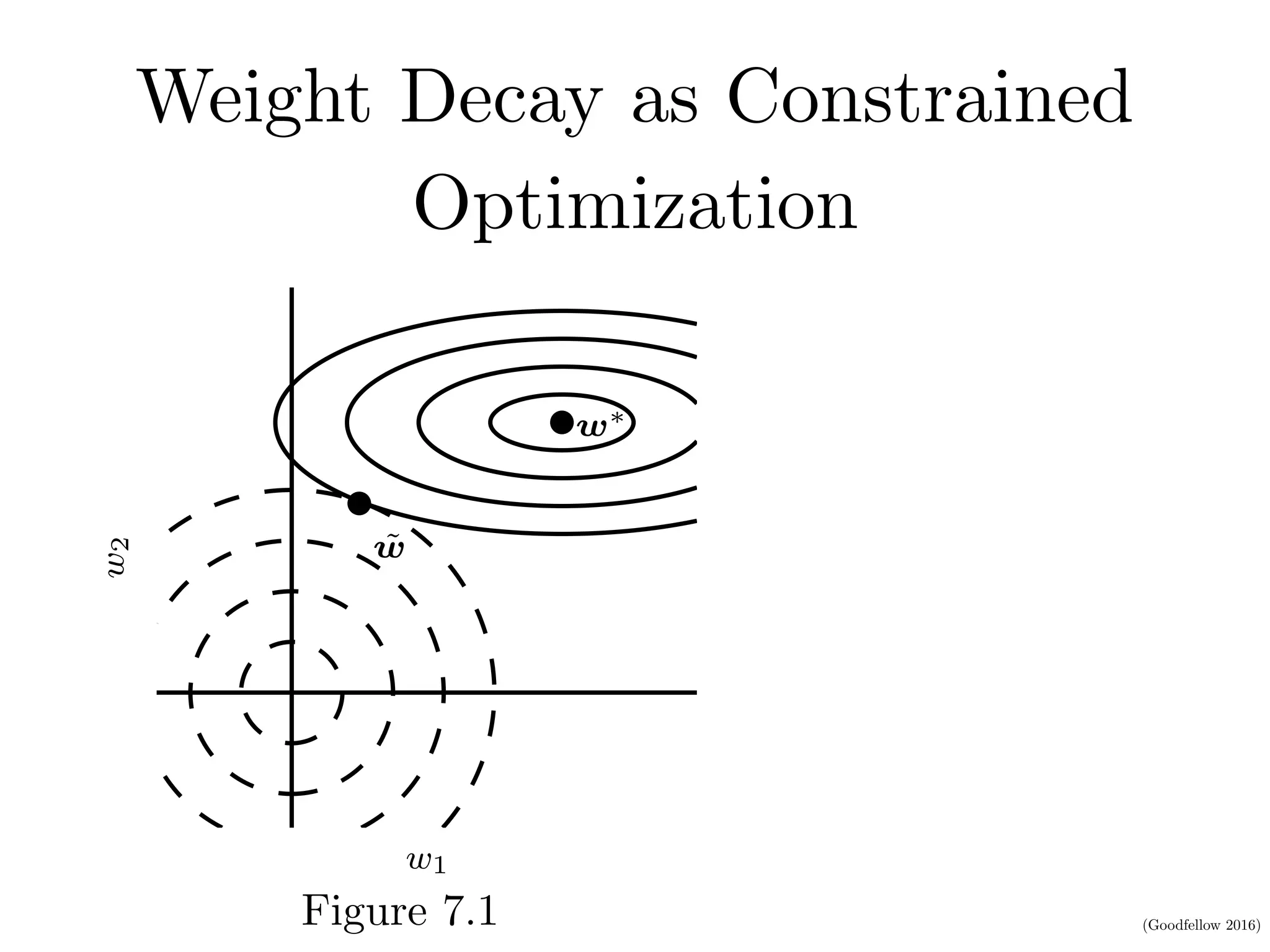
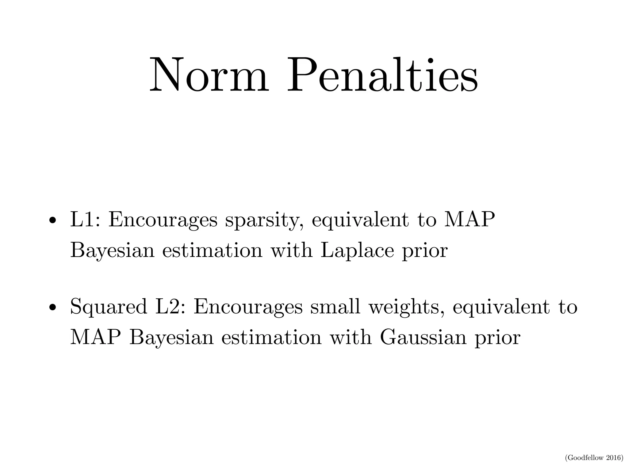
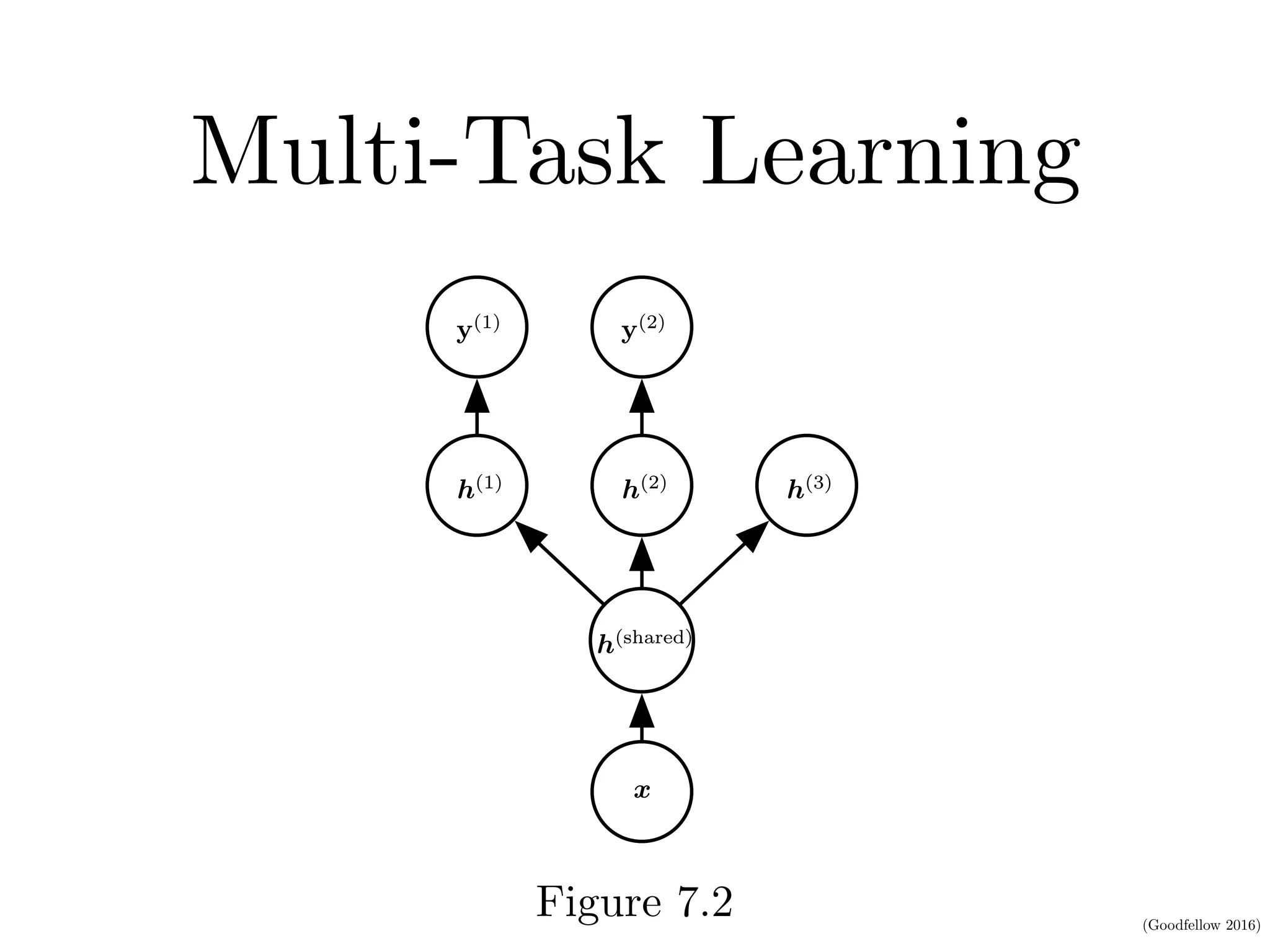
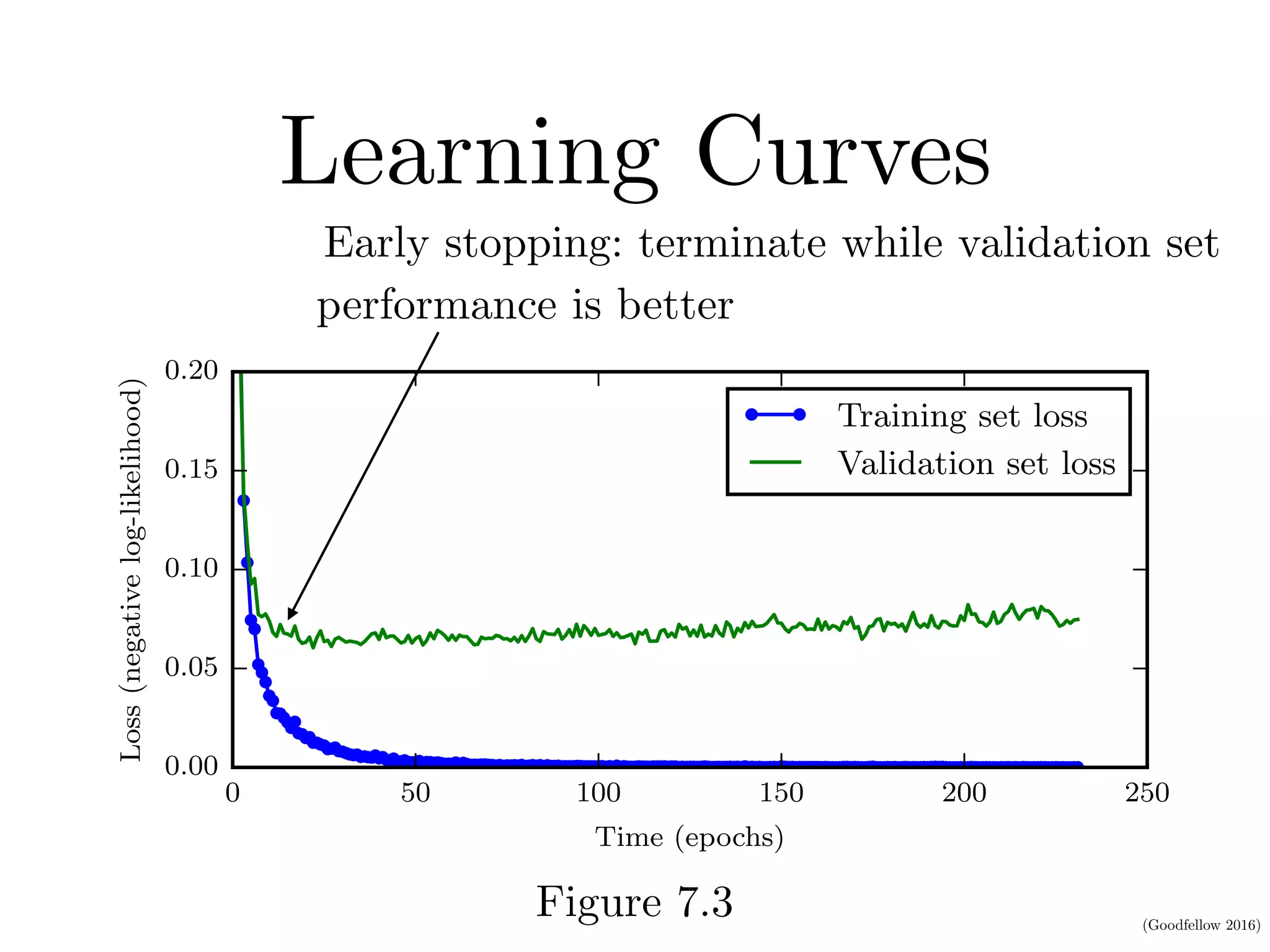
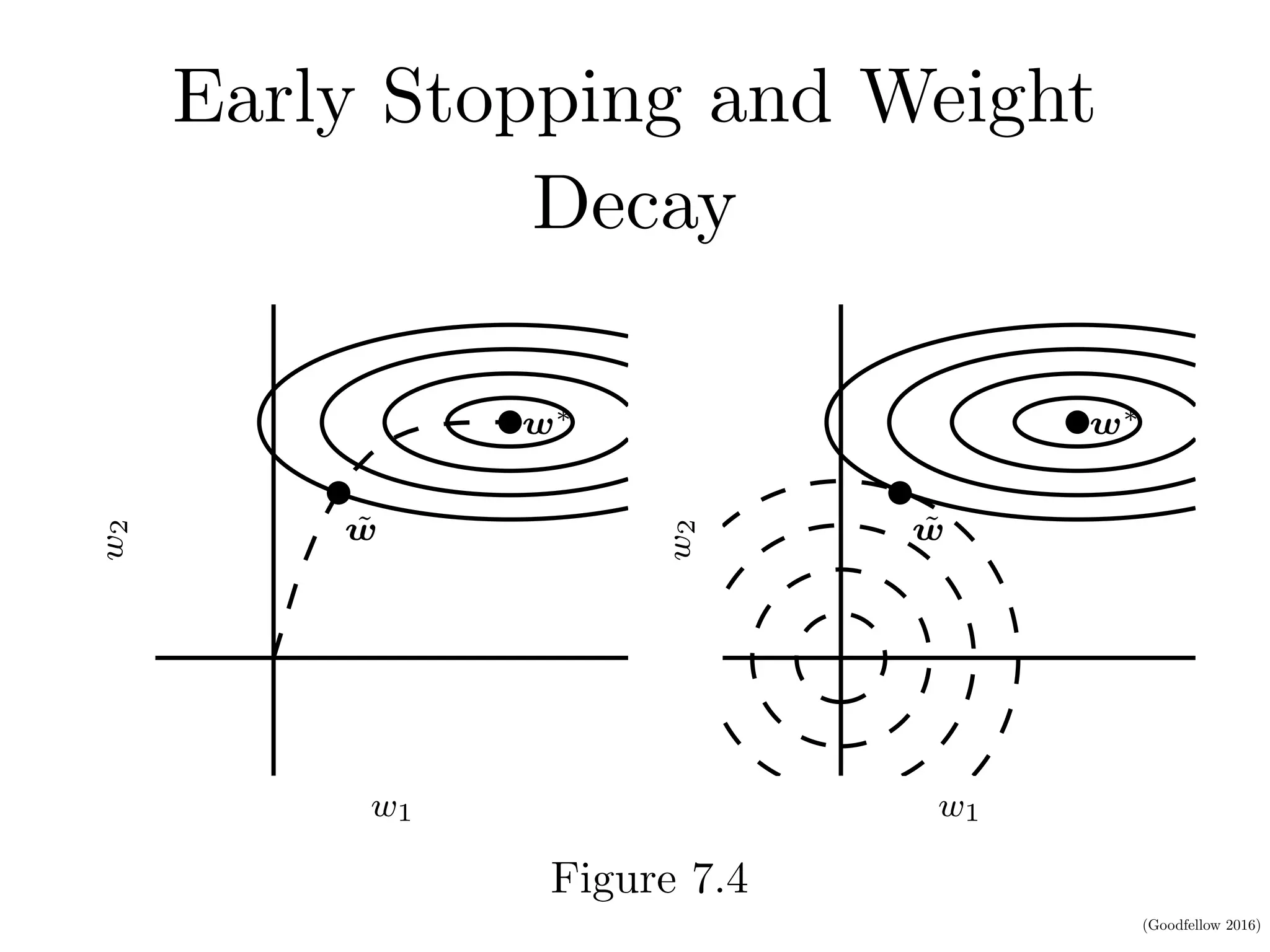
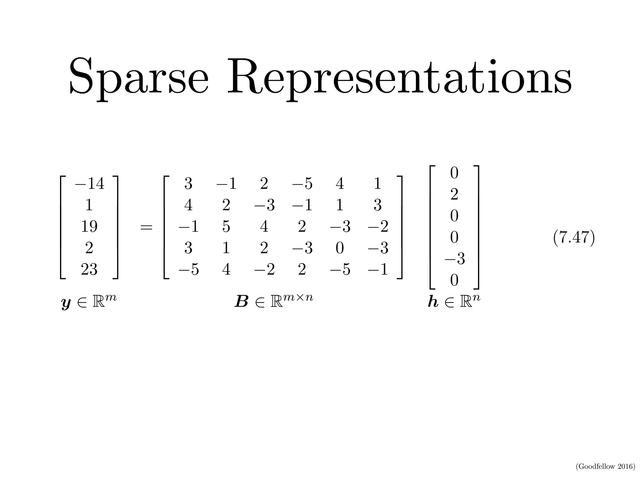
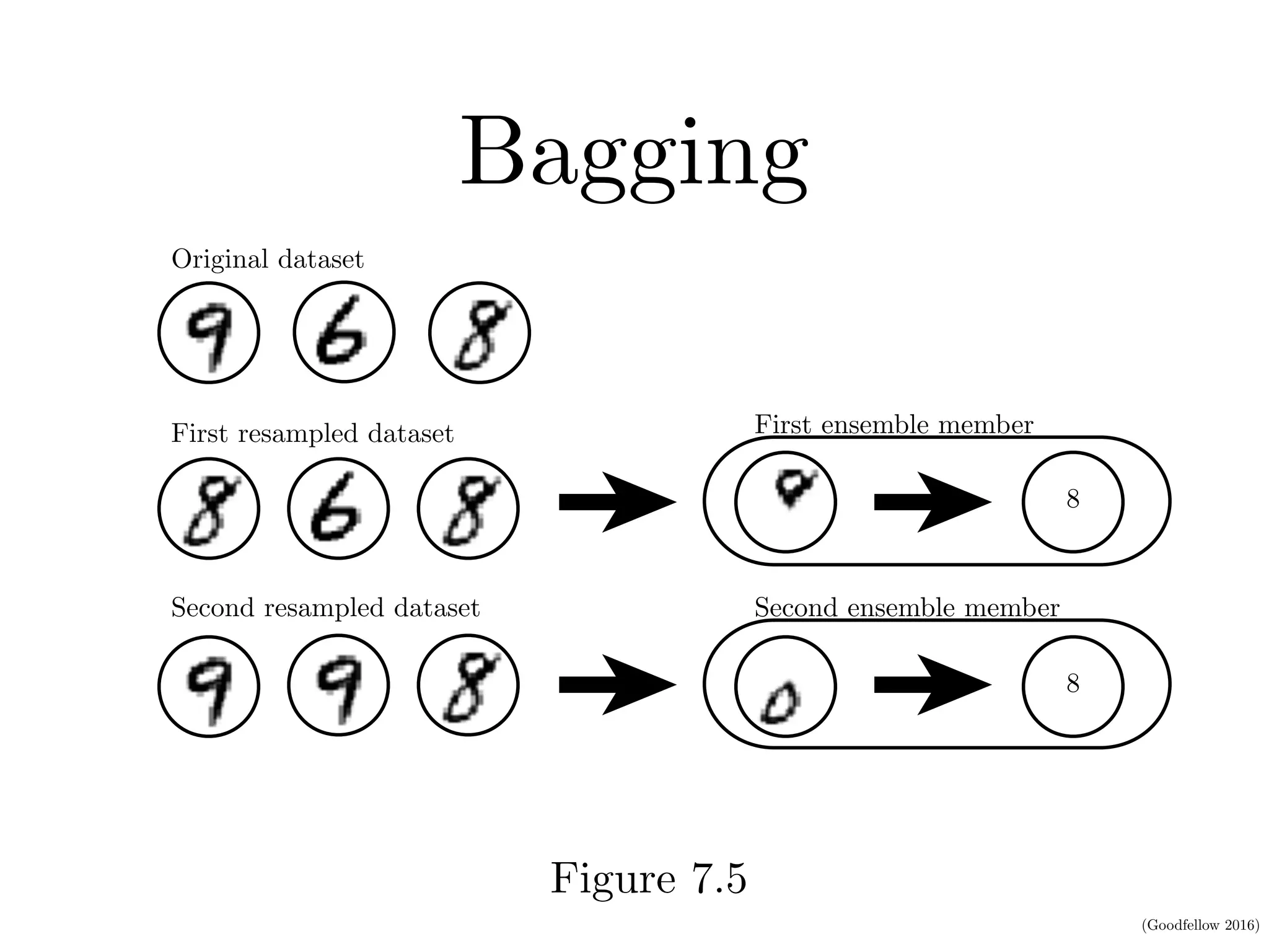
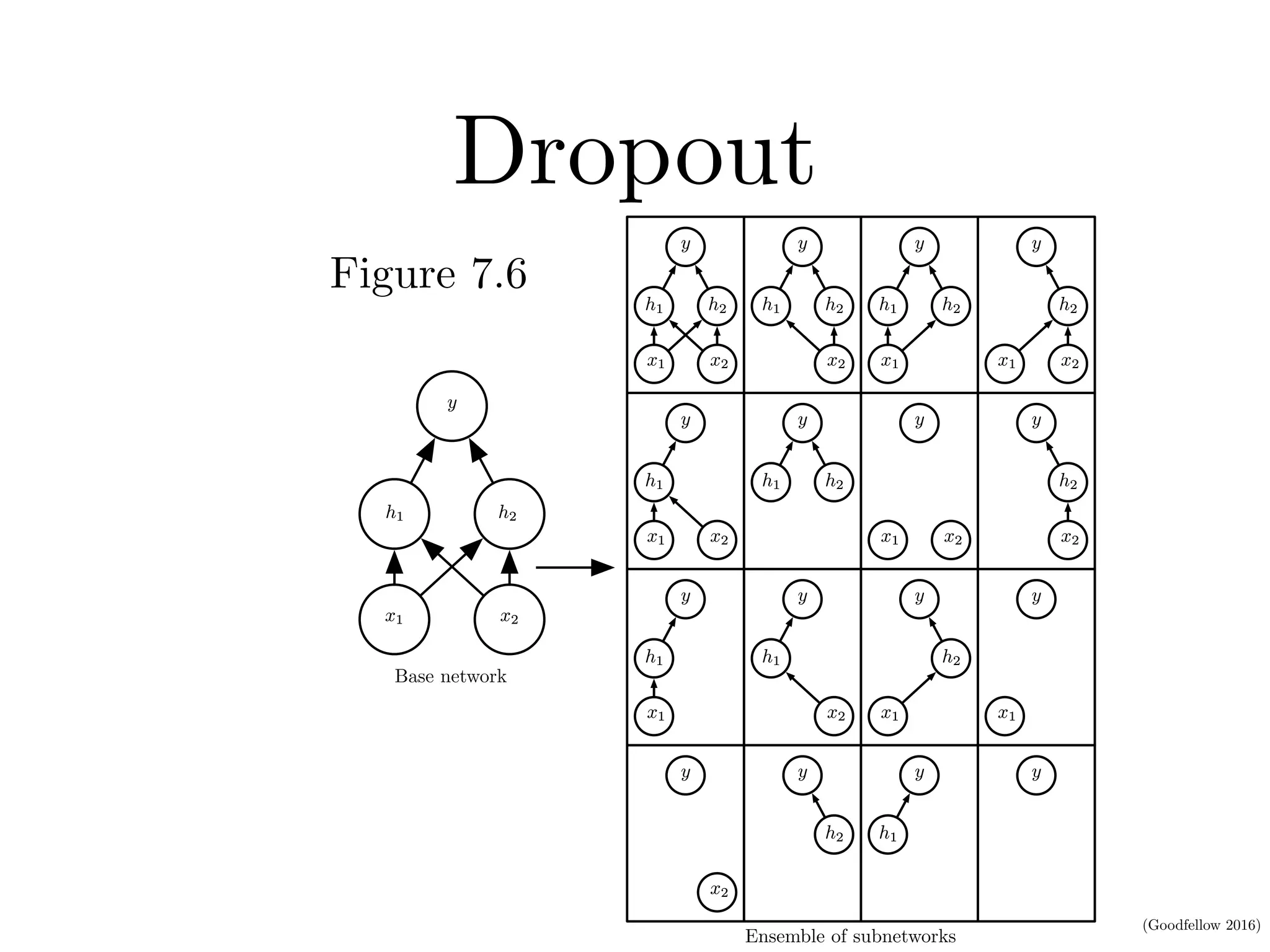
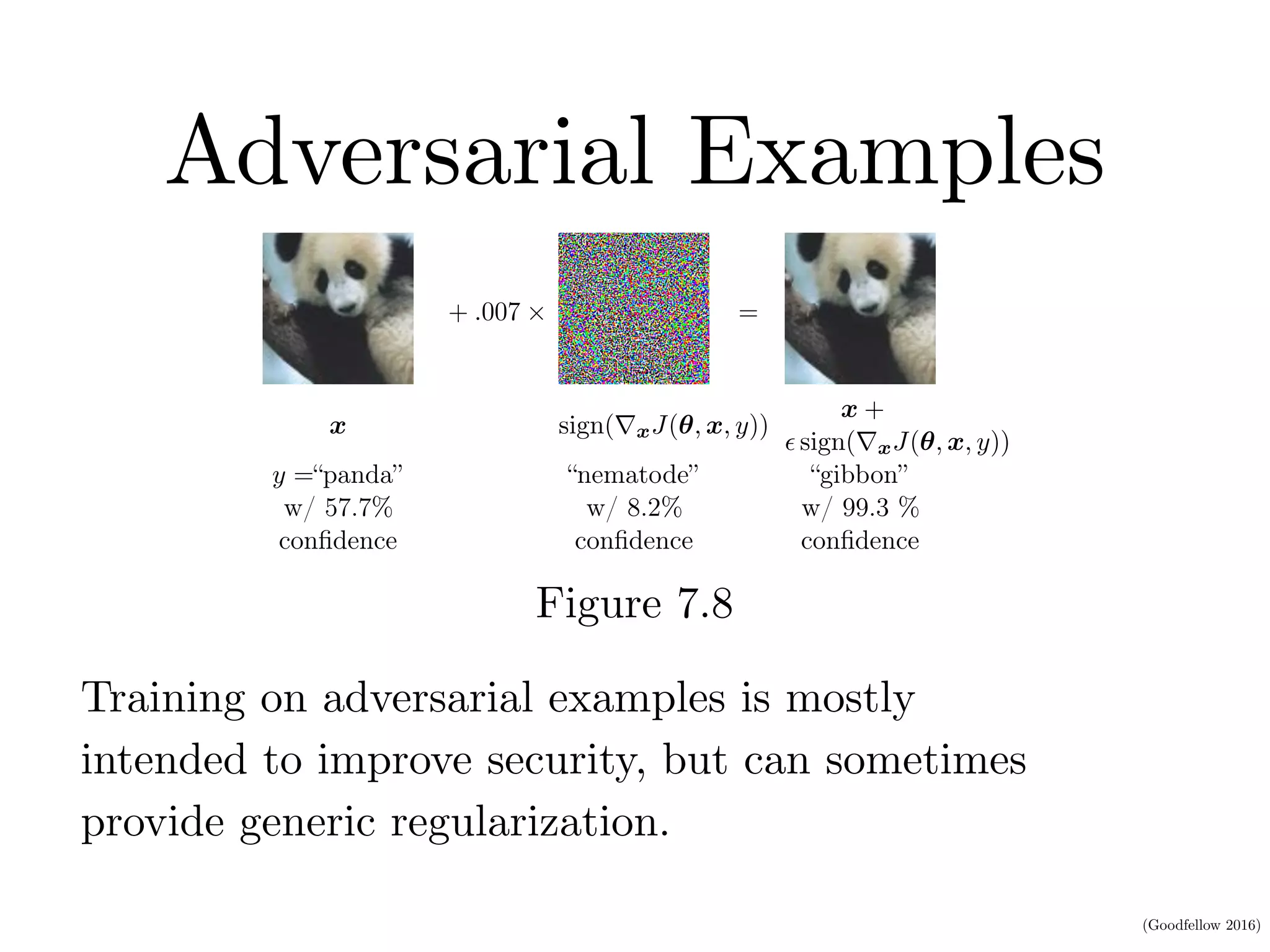
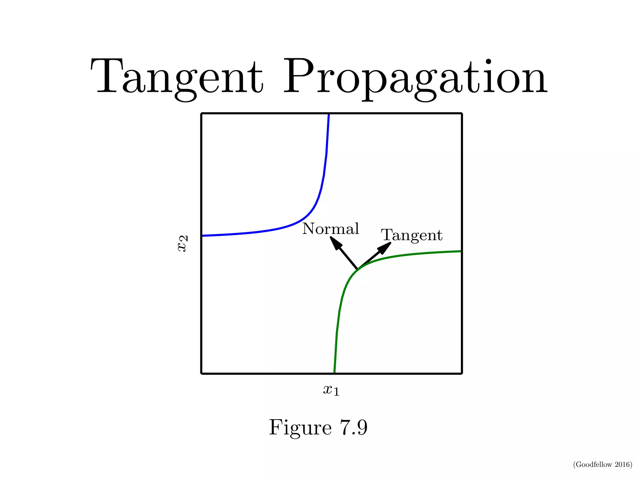
1. Regularization for
Deep Learning
Lecture slides for Chapter 7 of Deep Learning
www.deeplearningbook.org
Ian Goodfellow
2016-09-27

2. (Goodfellow 2016)
Definition
• “Regularization is any modification we make to a
learning algorithm that is intended to reduce its
generalization error but not its training error.”

3. (Goodfellow 2016)
Weight Decay as Constrained
Optimization
ARIZATION FOR DEEP LEARNING
w1
w2
w⇤
˜w
Figure 7.1

4. (Goodfellow 2016)
Norm Penalties
• L1: Encourages sparsity, equivalent to MAP
Bayesian estimation with Laplace prior
• Squared L2: Encourages small weights, equivalent to
MAP Bayesian estimation with Gaussian prior

5. (Goodfellow 2016)
Dataset Augmentation
Affine
Distortion
Noise
Elastic
Deformation
Horizontal
flip
Random
Translation
Hue Shift

6. (Goodfellow 2016)
Multi-Task Learning
network in figure 7.2.
2. Generic parameters, shared across all the tasks (which benefit from th
pooled data of all the tasks). These are the lower layers of the neural networ
in figure 7.2.
h(1)
h(1)
h(2)
h(2)
h(3)
h(3)
y(1)
y(1)
y(2)
y(2)
h(shared)
h(shared)
xx
Figure 7.2: Multi-task learning can be cast in several ways in deep learning frameworFigure 7.2

7. (Goodfellow 2016)
Learning CurvesHAPTER 7. REGULARIZATION FOR DEEP LEARNING
0 50 100 150 200 250
Time (epochs)
0.00
0.05
0.10
0.15
0.20
Loss(negativelog-likelihood)
Training set loss
Validation set loss
gure 7.3: Learning curves showing how the negative log-likelihood loss changes o
Figure 7.3
Early stopping: terminate while validation set
performance is better

8. (Goodfellow 2016)
Early Stopping and Weight
Decay
R 7. REGULARIZATION FOR DEEP LEARNING
w1
w2
w⇤
˜w
w1
w2
w⇤
˜w
Figure 7.4

9. (Goodfellow 2016)
Sparse Representations
HAPTER 7. REGULARIZATION FOR DEEP LEARNING
2
6
6
6
6
4
14
1
19
2
23
3
7
7
7
7
5
=
2
6
6
6
6
4
3 1 2 5 4 1
4 2 3 1 1 3
1 5 4 2 3 2
3 1 2 3 0 3
5 4 2 2 5 1
3
7
7
7
7
5
2
6
6
6
6
6
6
4
0
2
0
0
3
0
3
7
7
7
7
7
7
5
y 2 Rm B 2 Rm⇥n h 2 Rn
(7.47)
In the first expression, we have an example of a sparsely parametrized linear
egression model. In the second, we have linear regression with a sparse representa-
on h of the data x. That is, h is a function of x that, in some sense, represents
he information present in x, but does so with a sparse vector.
Representational regularization is accomplished by the same sorts of mechanisms
hat we have used in parameter regularization.
Norm penalty regularization of representations is performed by adding to the

10. (Goodfellow 2016)
BaggingCHAPTER 7. REGULARIZATION FOR DEEP LEARNING
8
8
First ensemble member
Second ensemble member
Original dataset
First resampled dataset
Second resampled dataset
Figure 7.5: A cartoon depiction of how bagging works. Suppose we train an 8 detector
the dataset depicted above, containing an 8, a 6 and a 9. Suppose we make two differ
resampled datasets. The bagging training procedure is to construct each of these data
by sampling with replacement. The first dataset omits the 9 and repeats the 8. On t
Figure 7.5

11. (Goodfellow 2016)
Dropout
CHAPTER 7. REGULARIZATION FOR DEEP LEARNING
yy
h1h1 h2h2
x1x1 x2x2
yy
h1h1 h2h2
x1x1 x2x2
yy
h1h1 h2h2
x2x2
yy
h1h1 h2h2
x1x1
yy
h2h2
x1x1 x2x2
yy
h1h1
x1x1 x2x2
yy
h1h1 h2h2
yy
x1x1 x2x2
yy
h2h2
x2x2
yy
h1h1
x1x1
yy
h1h1
x2x2
yy
h2h2
x1x1
yy
x1x1
yy
x2x2
yy
h2h2
yy
h1h1
yy
Base network
Ensemble of subnetworks
Figure 7.6

12. (Goodfellow 2016)
Adversarial ExamplesCHAPTER 7. REGULARIZATION FOR DEEP LEARNING
+ .007 ⇥ =
x sign(rxJ(✓, x, y))
x +
✏ sign(rxJ(✓, x, y))
y =“panda” “nematode” “gibbon”
w/ 57.7%
confidence
w/ 8.2%
confidence
w/ 99.3 %
confidence
Figure 7.8: A demonstration of adversarial example generation applied to GoogLeNet
(Szegedy et al., 2014a) on ImageNet. By adding an imperceptibly small vector whose
elements are equal to the sign of the elements of the gradient of the cost function with
respect to the input, we can change GoogLeNet’s classification of the image. Reproduced
with permission from Goodfellow et al. (2014b).
to optimize. Unfortunately, the value of a linear function can change very rapidly
if it has numerous inputs. If we change each input by ✏, then a linear function
with weights w can change by as much as ✏||w||1, which can be a very large
amount if w is high-dimensional. Adversarial training discourages this highly
sensitive locally linear behavior by encouraging the network to be locally constant
Figure 7.8
Training on adversarial examples is mostly
intended to improve security, but can sometimes
provide generic regularization.

13. (Goodfellow 2016)
Tangent Propagation
ER 7. REGULARIZATION FOR DEEP LEARNING
x1
x2
Normal Tangent
7.9: Illustration of the main idea of the tangent prop algorithm (Sima
nd manifold tangent classifier (Rifai et al., 2011c), which both regul
Figure 7.9