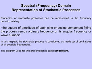
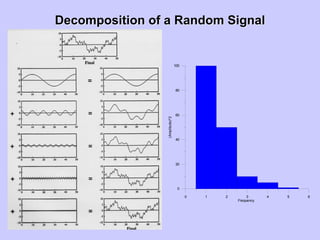
- The document discusses representation of stochastic processes in real and spectral domains and Monte Carlo sampling. - Stochastic processes can be represented in the real (time or space) domain using autocorrelation and variogram functions, and in the spectral domain using power spectral density functions. - Monte Carlo sampling uses techniques to generate random numbers from a probability density function for random sampling.

1. Lecture (2)Lecture (2)
RepresentationRepresentation
ofof Stochastic Processes inStochastic Processes in
Real and Spectral DomainsReal and Spectral Domains
andand
MonteMonte--Carlo samplingCarlo sampling

2. Summary of Lecture (1)Summary of Lecture (1)
•• Data types:[series or spatial (2D and 3DData types:[series or spatial (2D and 3D
Data)].Data)].
•• Axioms of probability of single and multiAxioms of probability of single and multi--
variatesvariates:[single::[single: pdfpdf,, cdfcdf
multimulti--variatevariate:: jpdfjpdf,, cdfcdf,, cpdfcpdf,, mdfmdf andand cmdfcmdf].].
•• Spatial and ensemble averagesSpatial and ensemble averages
[mean,variance and covariance].[mean,variance and covariance].
•• Basic terminology in the theory of stochasticBasic terminology in the theory of stochastic
modelling:[modelling:[StationarityStationarity,non,non--stationaritystationarity,,
intrinsic hypothesis andintrinsic hypothesis and ergodicityergodicity..

3. TopicsTopics
•• Representation of the stochastic process in real (timeRepresentation of the stochastic process in real (time
or space) domain:or space) domain:
AutoAuto--correlation andcorrelation and variogramvariogram..
•• Representation of the stochastic process in spectralRepresentation of the stochastic process in spectral
domain:domain:
Power spectral density functions.Power spectral density functions.
•• Random sampling in MonteRandom sampling in Monte--Carlo approach:Carlo approach:
Techniques of generating random numbers from aTechniques of generating random numbers from a
pdfpdf..

4. Real (Lag) Domain RepresentationReal (Lag) Domain Representation
of Stochastic Processesof Stochastic Processes
Properties of stationary stochastic processes may be
represented in a lag domain:
- auto-correlation function of the lag s, or
- cross-correlation function of s.
Correlogram: represents correlation coefficients
between values of the process versus the lag s.

5. Correlation, AutoCorrelation, Auto--Correlation and CrossCorrelation and Cross--
CorrelationCorrelation
Permeability, mD Permeability, mD
0 10 20 30
Porosity, %
Well No. 1 Well No. 1 Well No. 2
Sample Space
for Permeability
Sample Space
for Porosity
Correlation
Zone A
Zone B
Zone C
Crosscorrelation
Autocorrelation
10 -2 10 -1 10 0 10 1 10 2 10 310 -2 10 -1 10 0 10 1 10 2 10 3

6. Spatial AutoSpatial Auto--CorrelationCorrelation
It is a measure of the spatial correlation structure of a process.
( )
2
( )
1
( ), ( )
( )
1
( ( ), ( )) ( ) - ( ) -
( )
ZZ
Z
n
i i i j i i j i
j
Cov Z Z
Cov Z Z Z Z Z Z
n
ρ
σ
=
=
⎡ ⎤ ⎡ ⎤= ⎣ ⎦ ⎣ ⎦∑
s
x + s x
s
x + s x + sx x
s
The auto-correlation function has
the following properties:
)(-=)(
0)(
1)0(
ZZ ss ρρ
∞ρ
ρ
ZZ
ZZ
ZZ
=
=
,
,
i
j
X
Y
0
Z
Z
sij
1
p
,
,
,
2 3
,

7. Calculation of AutoCalculation of Auto--Correlation FunctionCorrelation Function
(1D)(1D)
[ ][ ]
σ
sCov
=sρ
Z-iZZ-siZ
sn
sCov
Z
x
xZZ
sn
i=
x
x
x
x
2
)(
1
)(
)(
)()(
)(
1
)( ∑ +=

8. Calculation of AutoCalculation of Auto--Correlation FunctionCorrelation Function
(2D)(2D)
X
Y0
< >
lag x=2dx
lag y=2dy
[ ][ ]
σ
ssCov
=ssρ
Z-jiZZ-sjsiZ
snsm
ssCov
Z
yx
yxZZ
sn
j=
yx
sm
iyx
yx
yx
2
)(
1
)(
1
),(
),(
),(),(
)()(
1
),( ∑∑ ++=
=

9. High and Poor CorrelationsHigh and Poor Correlations

10. Some AutoSome Auto--Correlation of SeriesCorrelation of Series

11. AutoAuto--correlation Modelscorrelation Models
Auto-correlation models
2
)(
)(
1)(
⎟
⎠
⎞
⎜
⎝
⎛
λ
−
λ
−
=ρ
=ρ
λ
−=ρ
s
s
es
es
s
s
0 5 10 15 20 250 5 10 15 20 250 5 10 15 20 25

12. 2D Isotropic Exponential Auto Correlation2D Isotropic Exponential Auto Correlation
⎥
⎥
⎦
⎤
⎢
⎢
⎣
⎡
⎟
⎟
⎠
⎞
⎜
⎜
⎝
⎛
λ
+
−=ρ
−
2/1
2
22
exp)(
var.exp.2
yx ss
ianceCoIstorpicD
s

13. Statistical Isotropy and AnisotropyStatistical Isotropy and Anisotropy
A multi-dimensional stochastic process is said to be
Isotropic, if the process does not have a preferred direction
, i.e., the variability in the process is the same in all directions.
Anisotropic, if the variability changes from one direction to another.
Isotropic Anisotropic

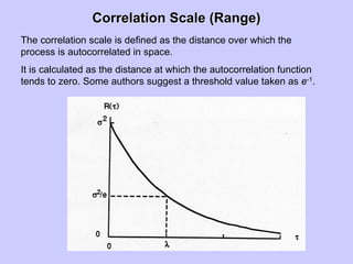
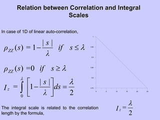
14. Integral ScaleIntegral Scale
The integral scale Iz of autocorrelation function is defined as,
0 5 10 15 20 25
0
0.2
0.4
0.6
0.8
1
∫
∞
0
)( ss dρ=I ZZz
which implies that the average distance over which the process is
autocorrelated in space.
For practical applications, the integration is calculated over a certain limits [0,
So] where, So is the smallest value of s at which the autocorrelation function
becomes practically zero.

15. Correlation Scale (Range)Correlation Scale (Range)
The correlation scale is defined as the distance over which the
process is autocorrelated in space.
It is calculated as the distance at which the autocorrelation function
tends to zero. Some authors suggest a threshold value taken as e-1.

16. Relation between Correlation and IntegralRelation between Correlation and Integral
ScalesScales
In case of 1D of linear auto-correlation,
∫ =⎥⎦
⎤
⎢⎣
⎡
−
≥
≤−
λ
λ
λ
λ
0
2
1
0)(
1)(
ds
λ
| s |
=I
sif=sρ
sif
λ
| s |
=sρ
z
ZZ
ZZ
The integral scale is related to the correlation
length by the formula, 2
λ
=I z
0 5 10 15 20 25
0.75
0.8
0.85
0.9
0.95
1

17. Examples of relations between correlationExamples of relations between correlation
and integral scalesand integral scales
λ=
⎪
⎩
⎪
⎨
⎧
λ>
λ<⎟
⎠
⎞
⎜
⎝
⎛
λ
+⎟
⎠
⎞
⎜
⎝
⎛
λ
−=ρ
π
λ
==ρ
λ
==ρ
λ
−
λ
−
8
3
.......................................0
............
2
1
2
3
1)(
2
,)(
2
,)(
3
2
2
z
z
s
z
s
I
s
s
ss
s
Ies
Ies

18. Spatial CrossSpatial Cross--CorrelationCorrelation
1/ 22 2
( ( ), ( ))
( )
( )
ZY
Z Y
Cov Z Y
sρ
σ σ
=
x +s x
The spatial cross-correlation represents a relation between two stochastic
processes. It defines the degree of which two stochastic process are correlated
as a function of separation lag.
positive or
negative or
zero

19. CrossCross--CorrelationCorrelation
( )
2
( )
1
( ), ( )
( )
1
( ( ), ( )) ( ) - ( ) -
( )
ZY
Z
n
i i i j i i j i
j
Cov Z Y
Cov Z Y Z Z Y Y
n
ρ
σ
=
=
⎡ ⎤ ⎡ ⎤= +⎣ ⎦ ⎣ ⎦∑
s
x + s x
s
x + s x sx x
s

20. AutoAuto--correlation of a Stationary Medium (1)correlation of a Stationary Medium (1)
myxm 25.0,1 =∆=∆=λ
0 5 10 15 20 25 30 35 40 45 50
-25
-20
-15
-10
-5
0
0 5 10 15 20 25 30 35 40 45 50
-25
-20
-15
-10
-5
0
-5.5
-3.5
-1.5
0.5
2.5
4.5
0
0.01
0.1
1
10

21. AutoAuto--correlation of a stationary Medium (1’)correlation of a stationary Medium (1’)
0 10 20 30 40 50
0
0.4
0.8
1.2
1/ 22 2
2
2 .exp. var
( ) exp x y
D Isotropic Co iance
s s
−
⎡ ⎤⎛ ⎞+
⎢ ⎥= −⎜ ⎟⎜ ⎟⎢ ⎥⎝ ⎠⎣ ⎦
ρ
λ
s
0 10 20 30 40 50
0
0.4
0.8
1.2
Single Realization Ensemble=70
myxm 25.0,1 =∆=∆=λ

22. AutoAuto--correlation of a Stationary Medium (2)correlation of a Stationary Medium (2)
myxm 25.0,5 =∆=∆=λ
0 5 10 15 20 25 30 35 40 45 50
-25
-20
-15
-10
-5
0
0 5 10 15 20 25 30 35 40 45 50
-25
-20
-15
-10
-5
0
-5.5
-3.5
-1.5
0.5
2.5
4.5
0
0.01
0.1
1
10

23. AutoAuto--correlation of a stationary Medium (2’)correlation of a stationary Medium (2’)
1/ 22 2
2
2 .exp. var
( ) exp
x y
D Isotropic Co iance
s s
−
⎡ ⎤⎛ ⎞+
⎢ ⎥ρ = −⎜ ⎟⎜ ⎟λ⎢ ⎥⎝ ⎠⎣ ⎦
s
0 10 20 30 40 50
0
0.4
0.8
1.2
0 10 20 30 40 50
0
0.4
0.8
1.2
Single Realization Ensemble=10
myxm 25.0,5 =∆=∆=λ

24. AutoAuto--correlation of a stationary Medium (3)correlation of a stationary Medium (3)
myxmm yx 25.0,5,25 =∆=∆=λ=λ
0 5 10 15 20 25 30 35 40 45 50
-25
-20
-15
-10
-5
0
0 5 10 15 20 25 30 35 40 45 50
-25
-20
-15
-10
-5
0
-7
-3.5
-1.5
0.5
2.5
4.5
0
0.01
0.1
1
10

25. AutoAuto--correlation of a Stationary Medium (3’)correlation of a Stationary Medium (3’)
Single Realization
Ensemble=10
myxmm yx 25.0,5,25 =∆=∆=λ=λ
1/ 2
22
2 2
2 .exp. var
( ) exp
yx
x y
D Anisotropic Co iance
ss
−
⎡ ⎤⎧ ⎫⎛ ⎞⎛ ⎞⎪ ⎪⎢ ⎥ρ = − + ⎜ ⎟⎨ ⎬⎜ ⎟ ⎜ ⎟⎢ ⎥λ λ⎝ ⎠⎪ ⎪⎝ ⎠⎩ ⎭⎣ ⎦
s
0 10 20 30 40 50
0
0.4
0.8
1.2
0 10 20 30 40 50
0
0.4
0.8
1.2

26. Rules of ThumpRules of Thump
4 ~ 5
(20 ~ 25)
x
x x
x
L
λ
λ
∆ ≤
≥

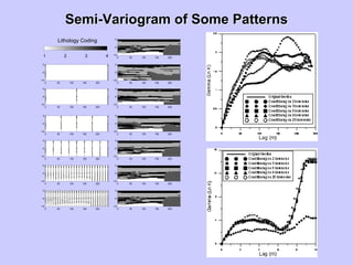
27. TheThe VariogramVariogram
Variogram: is a measure of variability between two quantities
Z(x) and Z(x+s) at two points at x and x+s separated by a
vector s.
[ ]
( )
2
1
1
( ) ( )- ( )
2 ( )
n
i
Z Z
n
γ
=
= ∑
s
s x +s x
s
n(s)=No. of pairs with lag s.

28. A TypicalA Typical VariogramVariogram

29. Nugget EffectNugget Effect
Definition:
It is the discontinuity of the variogram at the origin.
Interpretation:
1. Measurement errors.
2. Micro-variability is not accessible at the scale at
which the data are available they appear in the form of white
Noise.

30. How to Estimate SemiHow to Estimate Semi--VariogramVariogram from thefrom the
DataData
[ ]
( )
2
1
1
( ) ( )- ( )
2 ( )
n
i
Z Z
n
γ
=
= ∑
s
s x +s x
s
n(s)=No. of pairs with lag s
In words:
-Take all points with lag s.
-Take the difference in their values.
-Square the difference.
-Add up all the squares.
-Divide by twice the number of pairs.
-Repeat for other larger lag.

31. SemiSemi--VariogramVariogram Example Calculation (1)Example Calculation (1)
[ ]
( )
2
1
1
( ) ( )- ( )
2 ( )
n
i
Z Z
n
γ
=
= ∑
s
s x +s x
s
[ ]
[ ]
[ ]
[ ]
[ ]
[ ] 92.441625194
12
1
)4749()4650()4752()4950()5051()5254(
6*2
1
)3(
1.309990116
14
1
)4747()4649()4750()4952()5050()5251()5251()5054(
7*2
1
)2(
6.111414419
16
1
)4146...()5051()5154(
8*2
1
)1(
0)0(
222222
22222222
222
=+++++=
−+−+−+−+−+−=
=++++++=
−+−+−+−+−+−+−+−=
=+++++++=
−−+−=
=
γ
γ
γ
γ
0 1 2 3 4 5 6 7 8
46
47
48
49
50
51
52
53
54

32. SemiSemi--VariogramVariogram Example Calculation (2)Example Calculation (2)
[ ]
( )
2
1
1
( ) ( )- ( )
2 ( )
n
i
Z Z
n
γ
=
= ∑
s
s x +s x
s

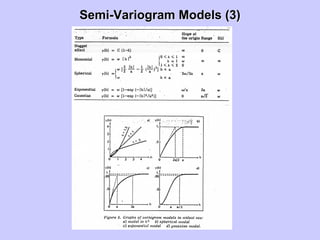
33. SemiSemi--VariogramVariogram Models (1)Models (1)
Semi-variogram models
sCsγ .)( =
]1[)( s
eCsγ −
−=
]1[)(
2s
s −
−= eCγ
]5.05.1[)( 3
ssCsγ −=
⎥⎦
⎤
⎢⎣
⎡
−=
s
s
Csγ
)sin(
1)(

34. SemiSemi--VariogramVariogram Models (2)Models (2)

35. SemiSemi--VariogramVariogram Models (3)Models (3)

36. SemiSemi--VariogramVariogram of a Compound Medium (1)of a Compound Medium (1)
0 50 100 150 200 250
-250
-200
-150
-100
-50
0
0 50 100 150 200 250
-250
-200
-150
-100
-50
0
0 50 100 150 200 250
-250
-200
-150
-100
-50
0
0 100 200 300
Spatial Lag (m)
0
1000
2000
3000
4000
Semi-Variogram(m/day)^2
X-direction
Small Scale Structure
Large Scale Structure
Two-Scales Structure

37. SemiSemi--VariogramVariogram of a Compound Medium (1’)of a Compound Medium (1’)
0 100 200 300
Spatial Lag (m)
0
1000
2000
3000
4000
5000
Semi-Variogram(m/day)^2
Y-direction
Small Scale Structure
Large Scale Structure
Two-Scales Structure
0 50 100 150 200 250
-250
-200
-150
-100
-50
0
0 50 100 150 200 250
-250
-200
-150
-100
-50
0
0 50 100 150 200 250
-250
-200
-150
-100
-50
0

38. SemiSemi--VariogramVariogram of a Compound Medium (2)of a Compound Medium (2)
0 100 200 300
Spatial Lag (m)
0
1000
2000
3000
4000
Semi-Variogram(m/day)^2
X-direction
Small Scale Structure
Large Scale Structure
Two Scales Structure
0 100 200
-200
-100
0
0 100 200
-200
-100
0
0 100 200
-200
-100
0

39. SemiSemi--VariogramVariogram of a Compound Medium (2’)of a Compound Medium (2’)

40. SemiSemi--VariogramVariogram of Some Patternsof Some Patterns
0 50 100 150 200
-10
-5
0
0 50 100 150 200
-10
-5
0
0 50 100 150 200
-10
-5
0
0 50 100 150 200
-10
-5
0
0 50 100 150 200
-10
-5
0
0 50 100 150 200
-10
-5
0
0 50 100 150 200
-10
-5
0
0 50 100 150 200
-10
-5
0
0 50 100 150 200
-10
-5
0
0 50 100 150 200
-10
-5
0
0 50 100 150 200
-10
-5
0
0 50 100 150 200
-10
-5
0
0 50 100 150 200
-10
-5
0
1 2 3 4
Lithology Coding

41. Spectral (Frequency) DomainSpectral (Frequency) Domain
Representation of Stochastic ProcessesRepresentation of Stochastic Processes
Properties of stochastic processes can be represented in the frequency
domain, relating:
“ the square of amplitude of each sine or cosine component fitting
the process versus ordinary frequency or its angular frequency or
wave number”.
In this respect, the stochastic process is considered as made up of oscillations
of all possible frequencies.
The diagram used for this presentation is called priodgram.

42. Decomposition of a Random SignalDecomposition of a Random Signal
0 1 2 3 4 5 6
Frequency
0
20
40
60
80
100
(Amplitude)^2

43. AutoAuto--Power (Variance) Spectral DensityPower (Variance) Spectral Density
Function (Function (AutoAuto--PSDPSD))
The term power is commonly seen in the literature. Its origin comes from the
field of electrical and communication engineering:
power dissipated in an electrical circuit is proportional to the mean square
voltage applied.
The adjective spectral denotes a function of frequency.
The concept of density comes from the division of the power (variance) of an
infinitesimal frequency interval by the width of that interval.
The power spectrum describes the distribution of power (variance) with
frequency of the random processes, and as such is real and non-negative.

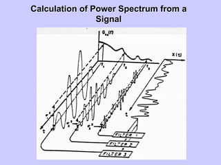
44. (Variance) Spectral Density Function(Variance) Spectral Density Function
The auto-power spectrum (spectral density function) for a process Z(x) is given
by,
[ ] ||z
L
=z.z
L
=S L
*
L
ZZ )(
1
lim)()(
1
lim)( 2
ωωωω
∞→∞→
where, z(ω) is Fourier transform of the process Z(x), which is expressed as,
0 5 10 15 20 250 5 10 15 20 25
0
5
10
15
20
25
0 5 10 15 20 25
deZ
π
=z -i
∫
∞
∞−
xxω xω
)(
2
1
)(
and z*(ω) is the conjugate of z(ω) and ω is the angular frequency vector.

45. Calculation of Power Spectrum from aCalculation of Power Spectrum from a
SignalSignal

46. Properties of the Spectral Density FunctionProperties of the Spectral Density Function
2
-
( ) 0
( )
( ) ( )
ZZ
ZZ Z
ZZ ZZ
S
dS
S S
σ
∞
∞
≥
=
= −
∫
ω
ω ω
ω ω

47. CrossCross--Power (Variance) Spectral DensityPower (Variance) Spectral Density
Function (Function (CrossCross--PSDPSD))
The cross-PSD is defined between a pair of stochastic process. Cross-PSD is
in general complex.
The magnitude of the cross-PSD describes whether frequency components in a
process are associated with large or small amplitudes at the same frequency in
another process, and the phase of the cross-PSD indicates the phase lag or
lead of one process with respect to the other one for a given frequency
component. This expressed mathematically as,
*1
( ) lim ( ). ( )ZY
L
z yS
L→∞
⎡ ⎤= ⎣ ⎦ω ω ω
where, y*(ω) is the conjugate of y(ω), and y(ω) is Fourier transform of the
process Y(x)

48. Relation betweenRelation between AutoCovarianceAutoCovariance FunctionsFunctions
andand AutoSpectralAutoSpectral Density FunctionsDensity Functions
The covariance functions and spectral density functions are Fourier transform
pairs. This can be expressed in mathematical forms using
Wiener-Khinchin relationships,
-
-
-
2
-
1
( ) ( )
2
( ) ( )
(0) ( )
i
ZZ ZZ
i
ZZ ZZ
ZZ ZZ Z
dS C e
dC S e
dC S
π
σ
∞
∞
∞
∞
∞
∞
=
=
= =
∫
∫
∫
ωs
ωs
ω s s
s ω ω
ω ω

49. Relation between Auto Correlation andRelation between Auto Correlation and
Power Spectrum (examples)Power Spectrum (examples)

50. Relation between CrossRelation between Cross--CovarianceCovariance
Functions and CrossFunctions and Cross--Spectral DensitySpectral Density
FunctionsFunctions
For cross-PSD and cross-correlation these relations are,
-
-
-
1
( ) ( )
2
( ) ( )
i
ZY ZY
i
ZY ZY
dS C e
dC S e
π
∞
∞
∞
∞
=
=
∫
∫
ωs
ωs
ω s s
s ω ω

51. Summary of A Random VariableSummary of A Random Variable

52. MonteMonte--Carlo SamplingCarlo Sampling
Uniform random number generator:
Multiplicative Congruence Method developed by Lehmer [1951].
/MN=U
MMODULOBNA.=N
or
B , MNA.= MODULON
ii
i-i
i-i
)()(
)(
1
1
+
+
Ni is a pseudo-random integer,
i is subscript of successive pseudo-random integers produced,
i-1 is the immediately preceding integer,
M is a large integer used as the modulus,
A and B are integer constants used to govern the relationship in company with
M,
Ui is a pseudo-random number in the range {0,1}, and
" MODULO" notation indicates that Ni is the remainder of the division of (A.Ni-1)
by M.

53. Uniform Random Number ExampleUniform Random Number Example
1.0,5.0,3.0,9.0
.......5,3,9,1,5,3,9:
)3(7
10
73
7319*8
)9(0
10
9
911*8
)1(4
10
41
4115*8
)5(2
10
25
2513*8
)3(7
10
73
7319*8
9)(
)10()18(
0
1
sequence
remainder
remainder
remainder
remainder
remainder
seedN
MODULON=N i-i
==+
==+
==+
==+
==+
=
+

54. Generation of a Random Variable from anyGeneration of a Random Variable from any
DistributionDistribution
Inverse of Distribution Function.
Transformation Method.
Acceptance-Rejection Method.

55. Inverse of Distribution FunctionInverse of Distribution Function
)(
)(
')'()(
UF=
F=U
αdαf=αF
1-
α
-
α
α
∫∞

56. Example of IDF in Discrete 1D Markov chainExample of IDF in Discrete 1D Markov chain
A B C D
A B C D
1,...n=l2,...n,=kpUp
k
q
lq
k
q
lq ,
1
1
1
∑∑ =
−
=
≤<

57. Transformation Method (1)Transformation Method (1)
Random number generator for normal distribution
(from central limit theory):" Observations which are the sum of many
independently operating processes tend to be normally distributed as the
number of effects becomes large"
12
2
1
m/
- m/U
ε =
m
i=
i∑
with mean (µ=0) and unit standard deviation (σ=1),
Ui is the i-th element of a sequence of random numbers from a uniform
distribution in the range {0,1}, and
m is the number of Ui to be used.
6
12
1
-Uε =
i
i∑=
If m is 12, a normal distribution with tails truncated at six times standard
deviation is produced
σ+ εµα = αα

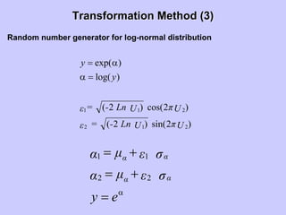
58. Transformation Method (2)Transformation Method (2)
Random number generator for normal distribution
Box and Muller method [1958].
)2sin()2(
)2cos()2(
212
211
UπULn-=ε
UπULn-=ε
where, U1 and U2 are independent random numbers distributed in the range
{0,1}, and
ε1 and ε2 are independent standard normally distributed random numbers with
zero mean (µ=0) and unit standard deviation (σ=1).
σε+µ=α
σε+µ=α
αα
αα
22
11

59. Transformation Method (3)Transformation Method (3)
Random number generator for log-normal distribution
)2sin()2(
)2cos()2(
)log(
)exp(
212
211
UπULn-=ε
UπULn-=ε
y
y
=α
α=
α
=
+=
+=
ey
σεµα
σεµα
αα
αα
22
11

60. Acceptance Rejection MethodAcceptance Rejection Method