The document discusses correlated and uncorrelated signals. It defines the inner product as a measure of how close two signals are to each other. The inner product calculates the correlation coefficient, which indicates whether signals are strongly correlated, uncorrelated, or anticorrelated. Matched filtering is introduced as a technique used in radar to detect the time delay of a received signal by sliding a transmitted pulse over the received signal and finding when the inner product is maximum.
![Correlated and Uncorrelated Signals
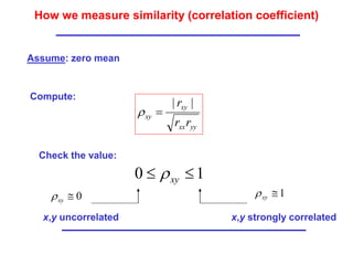
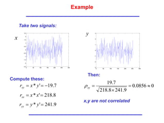
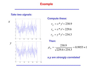
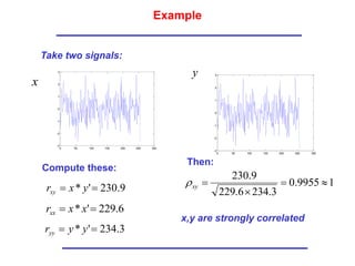
Problem: we have two signals and . How “close” are they to each other?
]
[n
x ]
[n
y
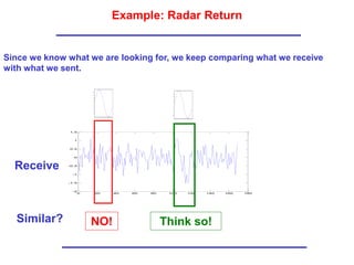
Example: in a radar (or sonar) we transmit a pulse and we expect a return
0 20 40 60 80 100 120 140 160 180
-2
-1.5
-1
-0.5
0
0.5
1
1.5
0 2 4 6 8 10 12 14 16 18 20
-1
-0.8
-0.6
-0.4
-0.2
0
0.2
0.4
0.6
0.8
1
Transmit
Receive](https://image.slidesharecdn.com/3-matched-filter-240214172034-28345fd5/85/3-Matched-Filter-ppt-1-320.jpg)
![Correlated and Uncorrelated Signals
Problem: we have two signals and . How “close” are they to each other?
]
[n
x ]
[n
y
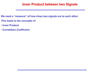
Example: in a radar (or sonar) we transmit a pulse and we expect a return
0 20 40 60 80 100 120 140 160 180
-2
-1.5
-1
-0.5
0
0.5
1
1.5
0 2 4 6 8 10 12 14 16 18 20
-1
-0.8
-0.6
-0.4
-0.2
0
0.2
0.4
0.6
0.8
1
Transmit
Receive](https://image.slidesharecdn.com/3-matched-filter-240214172034-28345fd5/75/3-Matched-Filter-ppt-1-2048.jpg)
![Inner Product
Problem: we have two signals and . How “close” are they to each other?
]
[n
x ]
[n
y
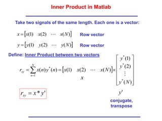
Define: Inner Product between two signals of the same length
1
0
*
]
[
]
[
N
n
xy n
y
n
x
r
Properties:
0
]
[
]
[
]
[
1
0
2
1
0
*
N
n
N
n
xx n
x
n
x
n
x
r
yy
xx
xy r
r
r
2
yy
xx
xy r
r
r
2
if and only if ]
[
]
[ n
x
C
n
y for some constant C](https://image.slidesharecdn.com/3-matched-filter-240214172034-28345fd5/85/3-Matched-Filter-ppt-4-320.jpg)
![003
.
0
982
500
27
.
2
xy
yy
xx
xy
r
r
r
Back to the Example: with no return
0 100 200 300 400 500 600 700 800 900
-2
-1.5
-1
-0.5
0
0.5
1
1.5
2
0 100 200 300 400 500 600 700 800 900
-3
-2
-1
0
1
2
3
0 100 200 300 400 500 600 700 800 900 1000
-3
-2
-1
0
1
2
3
]
[n
x ]
[n
y ]
[
]
[ n
y
n
x
NO Correlation!](https://image.slidesharecdn.com/3-matched-filter-240214172034-28345fd5/85/3-Matched-Filter-ppt-6-320.jpg)
![Back to the Example: with return
8
.
0
754
500
494
yy
xx
xy
r
r
r
0 100 200 300 400 500 600 700 800 900
-2
-1.5
-1
-0.5
0
0.5
1
1.5
2
0 100 200 300 400 500 600 700 800 900
-3
-2
-1
0
1
2
3
0 100 200 300 400 500 600 700 800 900 1000
-0.5
0
0.5
1
1.5
2
2.5
]
[n
x ]
[n
y ]
[
]
[ n
y
n
x
Good Correlation!](https://image.slidesharecdn.com/3-matched-filter-240214172034-28345fd5/85/3-Matched-Filter-ppt-7-320.jpg)
![Typical Application: Radar
]
[n
s
n
Send a Pulse…
]
[n
y
n
0
n
… and receive it back with noise, distortion …
N
Problem: estimate the time delay , ie detect when we receive it.
0
n](https://image.slidesharecdn.com/3-matched-filter-240214172034-28345fd5/85/3-Matched-Filter-ppt-12-320.jpg)
![Use Inner Product
“Slide” the pulse s[n] over the received signal and see when
the inner product is maximum:
]
[
s
]
[
y
0
n
N
n
1
0
*
]
[
]
[
]
[
N
ys s
n
y
n
r
0
if
,
0
]
[ n
n
n
rys
](https://image.slidesharecdn.com/3-matched-filter-240214172034-28345fd5/85/3-Matched-Filter-ppt-13-320.jpg)
![Use Inner Product
]
[
s
“Slide” the pulse x[n] over the received signal and see when
the inner product is maximum:
]
[
y
N
0
n
if 0
n
n
MAX
s
n
y
n
r
N
ys
1
0
*
]
[
]
[
]
[
](https://image.slidesharecdn.com/3-matched-filter-240214172034-28345fd5/85/3-Matched-Filter-ppt-14-320.jpg)
![Matched Filter
Take the expression
]
[
]
0
[
]
1
[
]
1
[
...
]
1
[
]
1
[
]
[
]
[
]
[
*
*
*
1
0
*
n
y
s
n
y
s
N
n
y
N
s
s
n
y
n
r
N
n
ys
Then
]
1
[
]
1
[
]
1
[
]
1
[
...
]
[
]
0
[
]
[
ˆ
N
n
y
N
h
n
y
h
n
y
h
n
r
]
[n
y ]
[n
h
1
,...,
0
],
1
[
]
[ *
N
n
n
N
s
n
h
]
1
[
]
[
ˆ
N
n
r
n
r ys
Compare this, with the output of the following FIR Filter](https://image.slidesharecdn.com/3-matched-filter-240214172034-28345fd5/85/3-Matched-Filter-ppt-15-320.jpg)
![Matched Filter
This Filter is called a Matched Filter
The output is maximum when
]
[n
y ]
[
ˆ n
r
]
[n
h
1
,...,
0
],
1
[
]
[ *
N
n
n
N
s
n
h
]
1
[
]
[
ˆ
N
n
r
n
r ys
0
1 n
N
n
1
0
N
n
n
i.e.](https://image.slidesharecdn.com/3-matched-filter-240214172034-28345fd5/85/3-Matched-Filter-ppt-16-320.jpg)
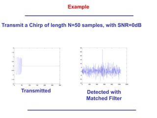
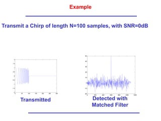
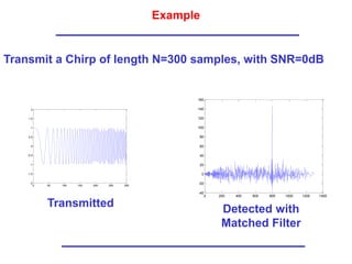
![Example
0 2 4 6 8 10 12 14 16 18 20
-1
-0.8
-0.6
-0.4
-0.2
0
0.2
0.4
0.6
0.8
1
]
[n
s
0 20 40 60 80 100 120 140 160 180 200
-6
-4
-2
0
2
4
6
8
10
12
0 20 40 60 80 100 120 140 160 180
-2
-1.5
-1
-0.5
0
0.5
1
1.5
]
[n
y
]
[n
y ]
[
ˆ n
r
]
[n
h
1
,...,
0
],
1
[
]
[ *
N
n
n
N
s
n
h
1
,...,
0
],
[
N
n
n
s
We transmit the pulse shown below, with
length 20
N
Received signal:
Max at n=119
100
1
20
119
0
n](https://image.slidesharecdn.com/3-matched-filter-240214172034-28345fd5/85/3-Matched-Filter-ppt-17-320.jpg)
![How do we choose a “good pulse”
1
,...,
0
],
[
N
n
n
s
We transmit the pulse and we receive
(ignore the noise for the time being)
]
[
]
[
]
[
]
[
0
1
0
*
0
n
n
r
A
s
n
n
s
A
n
r
ss
N
n
ys
]
[
]
[ 0
n
n
As
n
y
]
[
ˆ n
r
]
[n
h
1
,...,
0
],
1
[
]
[ *
N
n
n
N
s
n
h
]
1
[
]
[
ˆ
N
n
r
n
r ys
where
The term
is called the “autocorrelation of s[n]”. This characterizes
the pulse.
1
0
*
]
[
]
[
]
[
N
ss s
n
s
n
r
](https://image.slidesharecdn.com/3-matched-filter-240214172034-28345fd5/85/3-Matched-Filter-ppt-18-320.jpg)
![Example: a square pulse
?
]
[
]
[
]
[
1
0
*
N
ss s
n
s
n
r
N
s
s
s
r
N
N
ss
1
0
2
1
0
*
]
[
]
[
]
[
]
0
[
1
1
]
[
]
1
[
]
1
[
2
0
2
0
*
N
s
s
r
N
N
ss
k
N
s
k
s
k
r
k
N
k
N
ss
1
0
1
0
*
1
]
[
]
[
]
[
]
[n
rss
]
[n
s
n
1
N
1
0
N
N
N n
See a few values:
k
N
s
k
s
k
r
N
k
k
N
ss
1
1
0
*
1
]
[
]
[
]
[
](https://image.slidesharecdn.com/3-matched-filter-240214172034-28345fd5/85/3-Matched-Filter-ppt-19-320.jpg)
![Compute it in Matlab
]
[n
s
n
1
N
1
0
N=20; % data length
s=ones(1,N); % square pulse
rss=xcorr(s); % autocorr
n=-N+1:N-1; % indices for plot
stem(n,rss) % plot
-20 -15 -10 -5 0 5 10 15 20
0
2
4
6
8
10
12
14
16
18
20](https://image.slidesharecdn.com/3-matched-filter-240214172034-28345fd5/85/3-Matched-Filter-ppt-20-320.jpg)
![Example: Sinusoid
49
,...,
0
],
[
n
n
s
-50 -40 -30 -20 -10 0 10 20 30 40 50
-20
-15
-10
-5
0
5
10
15
20
25
0 5 10 15 20 25 30 35 40 45 50
-1
-0.8
-0.6
-0.4
-0.2
0
0.2
0.4
0.6
0.8
1
49
,...,
49
],
[
n
n
rss](https://image.slidesharecdn.com/3-matched-filter-240214172034-28345fd5/85/3-Matched-Filter-ppt-21-320.jpg)
![Example: Chirp
49
,...,
49
],
[
n
n
rss
49
,...,
0
],
[
n
n
s
0 5 10 15 20 25 30 35 40 45 50
-1
-0.8
-0.6
-0.4
-0.2
0
0.2
0.4
0.6
0.8
1
-50 -40 -30 -20 -10 0 10 20 30 40 50
-10
-5
0
5
10
15
20
25
30
s=chirp(0:49,0,49,0.1)](https://image.slidesharecdn.com/3-matched-filter-240214172034-28345fd5/85/3-Matched-Filter-ppt-22-320.jpg)
![Example: Pseudo Noise
49
,...,
49
],
[
n
n
rss
s=randn(1,50)
49
,...,
0
],
[
n
n
s
0 5 10 15 20 25 30 35 40 45 50
-2.5
-2
-1.5
-1
-0.5
0
0.5
1
1.5
2
2.5
-50 -40 -30 -20 -10 0 10 20 30 40 50
-20
-10
0
10
20
30
40
50](https://image.slidesharecdn.com/3-matched-filter-240214172034-28345fd5/85/3-Matched-Filter-ppt-23-320.jpg)
![Compare them
-50 -40 -30 -20 -10 0 10 20 30 40 50
-20
-10
0
10
20
30
40
50
-50 -40 -30 -20 -10 0 10 20 30 40 50
-10
-5
0
5
10
15
20
25
30
0 5 10 15 20 25 30 35 40 45 50
-2.5
-2
-1.5
-1
-0.5
0
0.5
1
1.5
2
2.5
0 5 10 15 20 25 30 35 40 45 50
-1
-0.8
-0.6
-0.4
-0.2
0
0.2
0.4
0.6
0.8
1
0 5 10 15 20 25 30 35 40 45 50
-1
-0.8
-0.6
-0.4
-0.2
0
0.2
0.4
0.6
0.8
1
-50 -40 -30 -20 -10 0 10 20 30 40 50
-20
-15
-10
-5
0
5
10
15
20
25
]
[n
s
]
[n
rss
cos chirp pseudonoise
Two best!](https://image.slidesharecdn.com/3-matched-filter-240214172034-28345fd5/85/3-Matched-Filter-ppt-24-320.jpg)
![Detection with Noise
Now see with added noise
]
[
]
[
]
[ 0 n
w
n
n
As
n
y
]
[n
h
1
,...,
0
],
1
[
]
[ *
N
n
n
N
s
n
h
]
[
]
1
[
]
[
ˆ 0 n
r
N
n
n
r
n
r yw
ys
](https://image.slidesharecdn.com/3-matched-filter-240214172034-28345fd5/85/3-Matched-Filter-ppt-25-320.jpg)
![White Noise
A first approximation of a disturbance is by “White Noise”.
White noise is such that any two different samples are
uncorrelated with each other:
0 100 200 300 400 500 600 700 800 900 1000
-4
-3
-2
-1
0
1
2
3
]
[n
w](https://image.slidesharecdn.com/3-matched-filter-240214172034-28345fd5/85/3-Matched-Filter-ppt-26-320.jpg)
![White Noise
The autocorrelation of a white noise signal tends to be a
“delta” function, ie it is always zero, apart from when n=0.
]
[n
rss
n](https://image.slidesharecdn.com/3-matched-filter-240214172034-28345fd5/85/3-Matched-Filter-ppt-27-320.jpg)
![White Noise and Filters
The output of a Filter
]
[n
w
]
[n
h
1
0
]
[
]
[
]
[
N
n
w
h
n
w
1
0
2
1
0
2
1
0
1
0
1
0
2
1
2
1
1
0
1
0
1
0
2
1
2
1
1
0
2
]
[
1
]
[
]
[
]
[
1
]
[
]
[
]
[
]
[
]
[
]
[
1
]
[
1
1 2
1 2
M
n
N
N N M
n
M
n
N N
M
n
n
w
M
h
n
w
n
w
M
h
h
n
w
n
w
h
h
M
n
w
M
](https://image.slidesharecdn.com/3-matched-filter-240214172034-28345fd5/85/3-Matched-Filter-ppt-28-320.jpg)
![White Noise
The output of a Filter
]
[n
w
]
[n
h
N
n
w
h
n
w
0
]
[
]
[
]
[
In other words the Power of the Noise at the ouput is
related to the Power of the Noise at the input as
w
N
n
W
P
n
h
P
1
0
2
]
[](https://image.slidesharecdn.com/3-matched-filter-240214172034-28345fd5/85/3-Matched-Filter-ppt-29-320.jpg)
![Back to the Match Filter
At the peak:
]
[
]
[
]
[ 0 n
w
n
n
As
n
y
]
[n
h
1
,...,
0
],
1
[
]
[ *
N
n
n
N
s
n
h
]
[
]
1
[
]
[
ˆ 0 n
w
N
n
n
Ar
n
r ss
]
1
[
]
0
[
]
1
[
ˆ 0
0
N
n
w
Ar
N
n
r ss](https://image.slidesharecdn.com/3-matched-filter-240214172034-28345fd5/85/3-Matched-Filter-ppt-30-320.jpg)
![Match Filter and SNR
At the peak:
]
1
[
]
0
[
]
1
[
ˆ 0
0
N
n
r
Ar
N
n
r sw
ss
1
0
2
1
0
2
2
|
]
[
|
|
]
[
|
]
0
[
N
n
N
n
ss n
s
n
As
Ar
W
N
n
W
P
n
s
P
1
0
2
|
]
[
|
SNR
N
P
n
s
n
s
P
N
SNR
W
N
n
N
n
S
peak
1
0
2
1
0
2
]
[
]
[](https://image.slidesharecdn.com/3-matched-filter-240214172034-28345fd5/85/3-Matched-Filter-ppt-31-320.jpg)