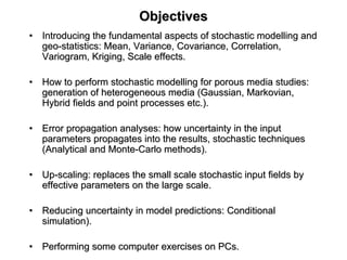
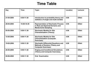
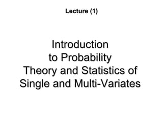
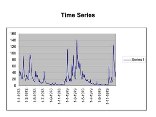
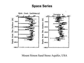
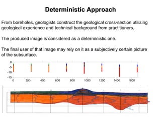
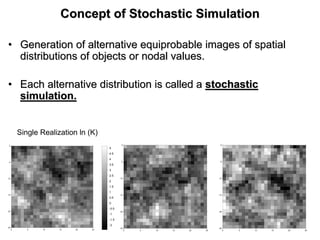
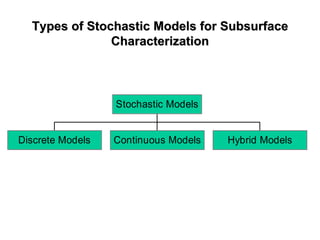
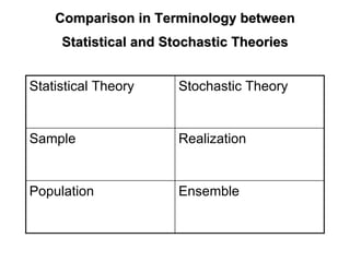
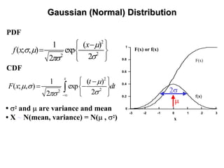
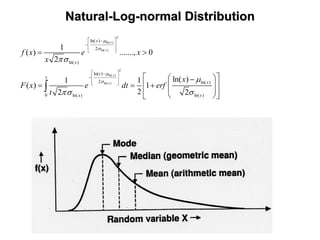
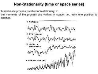
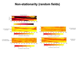
The document outlines the fundamentals of stochastic hydrology, including models for porous media, error propagation analyses, and methods for reducing uncertainty in model predictions. It introduces key concepts such as stochastic processes, geostatistics, and simulation techniques while providing a timetable for lectures and exercises. The document emphasizes the stochastic approach in evaluating spatial variability in hydrogeological parameters.


![Definition of Stochastic ProcessDefinition of Stochastic Process
•• A stochastic process may be defined, Bartlett [1960]:A stochastic process may be defined, Bartlett [1960]:
" a physical process in the real world, that has some random or" a physical process in the real world, that has some random or
stochastic element involved in its structures"stochastic element involved in its structures"
If a process is operating through time or space: it is considereIf a process is operating through time or space: it is considered asd as
system comprising a particular set of states:system comprising a particular set of states:
•• In a classical deterministic model:In a classical deterministic model: the state of the system inthe state of the system in
time or space can be exactly predicted from knowledge of thetime or space can be exactly predicted from knowledge of the
functional relation specified by the governing differentialfunctional relation specified by the governing differential
equations of the system (deterministic regularity).equations of the system (deterministic regularity).
•• In a stochastic model:In a stochastic model: the state of the system at any time orthe state of the system at any time or
space is characterized by the underling fixed probabilities of tspace is characterized by the underling fixed probabilities of thehe
states in the system (statistical regularity).states in the system (statistical regularity).](https://image.slidesharecdn.com/lecture1-190407221228/85/Stochastic-Hydrology-Lecture-1-Introduction-15-320.jpg)
![Historical BackgroundHistorical Background
•• Warren and Price [1961]: Stochastic model ofWarren and Price [1961]: Stochastic model of
macroscopic flow.macroscopic flow.
•• Warren and Price [1964]: Stochastic model ofWarren and Price [1964]: Stochastic model of
transport.transport.
•• Freeze [1975]: OneFreeze [1975]: One--dimensional groundwater flow.dimensional groundwater flow.
•• Freeze [1977]: OneFreeze [1977]: One--dimensional consolidationdimensional consolidation
problems.problems.
•• Revolution in stochastic subsurface heterogeneity.Revolution in stochastic subsurface heterogeneity.](https://image.slidesharecdn.com/lecture1-190407221228/85/Stochastic-Hydrology-Lecture-1-Introduction-29-320.jpg)
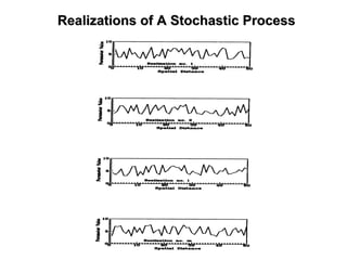
![Definition of The Stochastic ProcessDefinition of The Stochastic Process
A stochastic process can be defined as:
“a collection of random variables”.
In a mathematical form:
the set {[x, Z(x,ζi)], x ∈ Rn }, i = 1,2,3...,m.
Z(x,ζ) is stochastic process, (random function),
x is the coordinates of a point in n-dimensional space,
ζ is a state variable (the model parameter),
Z(x,ζi) represents one single realization of the stochastic process, i= 1,2,...,m
(i: realization no. of the stochastic process Z),
Z(x0,ζ) = random variable, i.e., the ensemble of the realizations of the
stochastic process Z at x0, and
Z(x0,ζi)= single value of Z at x0.
For simplification the variable ζ is generally omitted and the notation of this
stochastic process is Z(x).](https://image.slidesharecdn.com/lecture1-190407221228/85/Stochastic-Hydrology-Lecture-1-Introduction-32-320.jpg)
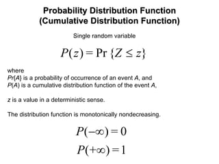
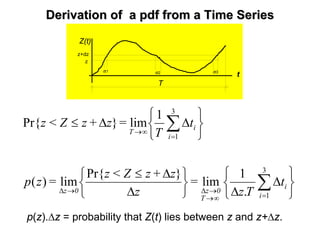
![Probability Density Function (PDF)Probability Density Function (PDF)
The density function, p(z), of random variable Z is defined by,
dz
zdP
=
z
z+zZ<z
=zp
z
)(}Pr{
lim)(
0 ∆
∆≤
→∆
Inversely, the distribution function can be expressed in terms of
the density function as follows
∫∞
z
-
dzzp=zP ')'()(
p(z) is not a probability, but must be multiplied by a certain region ∆z to obtain a
probability (i.e.: p(z).∆z).
P(z) is dimensionless, but p(z) is not. It has dimension of [z-1].](https://image.slidesharecdn.com/lecture1-190407221228/85/Stochastic-Hydrology-Lecture-1-Introduction-39-320.jpg)
![Uniform DistributionUniform Distribution
f(x) or F(x)
x
a b
1.0
0
F(x)
f(x)
(a-b)
1
1
( )f x
b a
=
−
[ ]
1 1
( )
x
a
F x dt x a
b a b a
= = −
− −∫
• Two parameter distribution
• Useful when only range is known](https://image.slidesharecdn.com/lecture1-190407221228/85/Stochastic-Hydrology-Lecture-1-Introduction-41-320.jpg)
![Exponential DistributionExponential Distribution
0
1
0
F(x)orf(x)
x
F(x)
f(x)
exp( ), 0
( )
0 otherwise
x x
f x
λ −λ ≥⎧
= ⎨
⎩
[ ]
0
( ) exp( ) 1 exp( )
x
F x t dt x= λ −λ = − −λ∫
•• One parameter modelOne parameter model
•• Useful for fracture spacingUseful for fracture spacing](https://image.slidesharecdn.com/lecture1-190407221228/85/Stochastic-Hydrology-Lecture-1-Introduction-44-320.jpg)
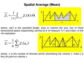
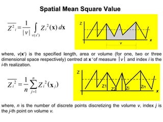
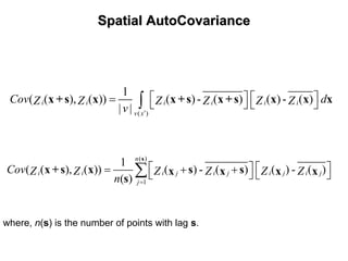
![Spatial VarianceSpatial Variance
where, v(x′) is the specified length, area or volume (for one, two or three
dimensional space respectively) centred at x′ of measure ⎮v⎮ and index i is the
i-th realization.
where, n is the number of discrete points discretizing the volume v, index j is
the j-th point on volume v.
2
2
2
( )
[ ] ( ) -
1
( ) -
| |
i
i i iZ
i i
v x
Var xZ Z ZS
x dxZ Z
v ′
⎡ ⎤= = ⎣ ⎦
⎡ ⎤= ⎣ ⎦∫
2
2
1
1
( ) -
-1i
n
i ijZ
j
xZ ZS
n =
⎡ ⎤= ⎣ ⎦∑
222
- ( )i i iZ
ZZS =
Z
x
v
Z
x
Z1-Z
Z2-Z Zi-Z
Zn-Z](https://image.slidesharecdn.com/lecture1-190407221228/85/Stochastic-Hydrology-Lecture-1-Introduction-59-320.jpg)
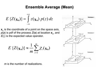
![Ensemble VarianceEnsemble Variance
[ ]{ } ( )
[ ]
( )
2 2
2
( )
2
2
( )
1
222
( )
( ) - { ( )} ( )( ) - { ( )}
1
( ) - { ( )}
{ ( )}- { ( )}
Z
m
iZ
i
Z
E Z E Z p z dzZ E Z
E ZZ
m
E E ZZ
σ
σ
σ
∞
−∞
=
= =
≈
=
∫
∑
o
o
o
o oo ox
o ox
o ox
x xx x
x x
x x](https://image.slidesharecdn.com/lecture1-190407221228/85/Stochastic-Hydrology-Lecture-1-Introduction-65-320.jpg)
![StationarityStationarity
,
,
i
j
X
Y
0
Z
Z
sij
1
p
,
,
,
2 3
,
The stochastic process is said to be second-order stationary (weak sense) if:
1) The mean value is constant at all points in the field, i.e., the mean
does not depend on the position.
{ ( )} ZE Z µ=x
2) The covariance depends only on the difference between the
position vectors of two points (xi-xj)= sij the separation vector, and does
not depend on the position vectors xi and xj themselves.
[ ]{ }( ( ), ( )) ( )- { ( )} ( ) - { ( )} ( )i j i i j jCov Z Z E Z E Z Z E Z Cov= =⎡ ⎤⎣ ⎦ sx x x x x x
[ ] 2
( ) (0) ZVar Z Cov σ= =x](https://image.slidesharecdn.com/lecture1-190407221228/85/Stochastic-Hydrology-Lecture-1-Introduction-69-320.jpg)
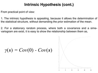
![Intrinsic HypothesisIntrinsic Hypothesis
The intrinsic hypothesis assumes that even if the variance of Z(x) is not finite,
the variance of the first-order increments of Z(x) is finite and these increments
are themselves second-order stationary.
This hypothesis postulates that:
(1) the mean is the same everywhere in the field; and
(2) for all distances, s, the variance of the increments, {Z(x+s)-Z(x)} is a
unique function of s so independent of x.
A stochastic process that satisfies the stationarity of order two also satisfies the
intrinsic hypothesis, but the converse is not true.
[ ]{ }2
{ ( )- ( )} 0
( )- ( ) 2 ( )
E Z Z
E Z Z γ
+ =
+ =
x s x
x s x s
γ(s) is called the semi-variogram,](https://image.slidesharecdn.com/lecture1-190407221228/85/Stochastic-Hydrology-Lecture-1-Introduction-72-320.jpg)
![Comparison between Intrinsic HypothesisComparison between Intrinsic Hypothesis
and Secondand Second--orderorder StationarityStationarity
Intrinsic Hypothesis Second-order
Stationarity
Less strict than 2nd
order stationarity
More strict than
Intrinsic hypothesis
Variogram Correlogram
If the phenomenon does not have a finite
variance, the variogram will never have a
horizontal asymptotic value.
{ ( )- ( )} 0E Z Z =x +s x { ( )} ZE Z µ=x
[ ]{ }21
( ) ( )- ( )
2
E Z Zγ =s x +s x [ ][ ]{ }( ) ( ) . ( )Z ZCov E Z Zµ µ= − −s x +s x
finitebemustσ Z
2](https://image.slidesharecdn.com/lecture1-190407221228/85/Stochastic-Hydrology-Lecture-1-Introduction-74-320.jpg)