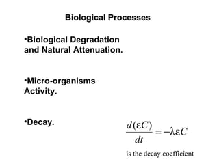
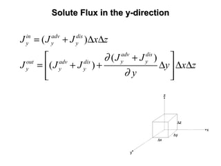
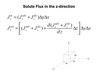
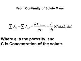
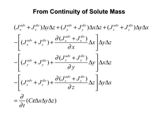
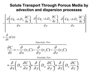
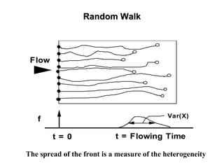
The lecture discusses transport processes in porous media, covering contaminant movement, concentration levels, and the derivation of the advective dispersion equation. It highlights physical, chemical, biological processes and methods of solution including analytical and numerical approaches. Key topics include advection, diffusion, dispersion, adsorption, and decay, with a focus on their effects on pollutant transport.

1. Lecture (2)Lecture (2)
Transport Processes in
Porous Media

2. Lecture (2)Lecture (2)
1. After how many years the contaminant reaches a river or a
water supply well?
2. What is the level of concentration at the well?

3. Layout of the LectureLayout of the Lecture
• Transport Processes in Porous Media.Transport Processes in Porous Media.
• Derivation of The Transport Equation (ADE).Derivation of The Transport Equation (ADE).
• Methods of Solution.Methods of Solution.
• Effect of Heterogeneity on Transport:Effect of Heterogeneity on Transport:
Laboratory Experiments (movie).Laboratory Experiments (movie).

4. Transport ProcessesTransport Processes
1)1) Physical :Physical :
Advection-Diffusion-DispersionAdvection-Diffusion-Dispersion
2) Chemical:2) Chemical:
Adsorption- Ion Exchange- etc.Adsorption- Ion Exchange- etc.
3) Biological:3) Biological:
Micro-organisms ActivityMicro-organisms Activity
(Bacteria&Microbes)(Bacteria&Microbes)
4) Decay:4) Decay:
Radioactive Decay-Natural Attenuation.Radioactive Decay-Natural Attenuation.

5. Physical ProcessesPhysical Processes
1. Advection
2. Molecular Diffusion
3. Mechanical Dispersion
4. Hydrodynamic Dispersion

6. Advection (Convection)Advection (Convection)
adv
J Cq=
Advective Solute Mass Flux:
.q = K− ∇Φ
is the advective solute mass flux,
is the solute concentration, and
is the water flux (specific discharge) given by Darcy's law:
C
q
adv
J

7. Molecular DiffusionMolecular Diffusion
Diffusive Flux in Bulk: (Fick’s Law of Diffusion)
is the diffusive solute mass flux in bulk,
dif
o oJ = - D C∇
dif
oJ
is the solute concentration gradient,C∇
is the molecular diffusive coefficient in bulk.oD
Random Particle motion
Time
t1
t2
t3
t4

8. Molecular Diffusion (Cont.)Molecular Diffusion (Cont.)
dif
effJ = - D C∇
τ
O
eff
D
D =
Diffusive Flux in Porous Medium
is the effective molecular diffusion
coefficient in porous medium,
effD
τ is a tortuosity factor ( = 1.4)
0.7eff oD D:

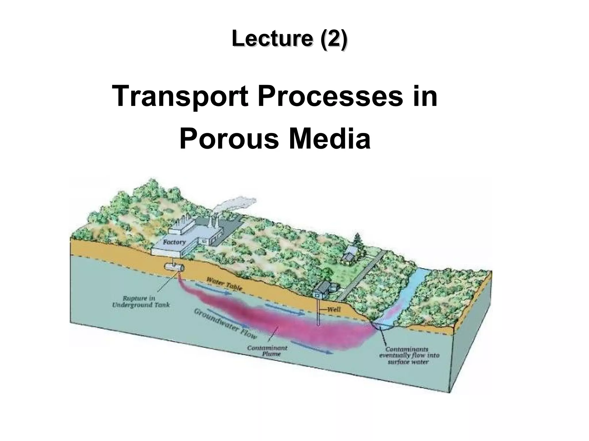
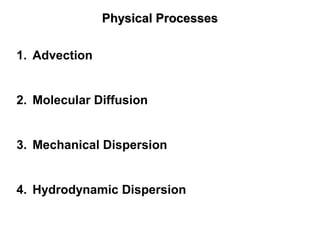
9. Mechanical DispersionMechanical Dispersion
dis
J = - Cε ∇.D
Depressive Flux in Porous Media (Fick’s Law):
is the depressive solute mass flux,
is the solute concentration gradient,
is the dispersion tensor,
is the effective porosity
dis
J
ε
C∇
D
xx xy xz
yx yy yz
zx zy zz
D D D
D D D
D D D
 
 
=  
 
 
D
[after Kinzelbach, 1986]
Causes of Mechanical Dispersion

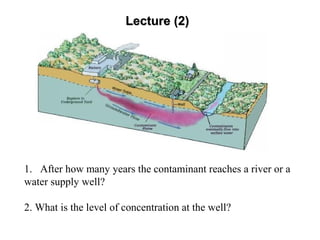
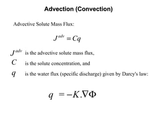
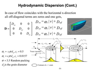
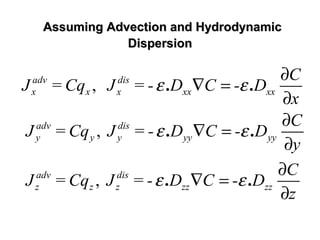
10. Hydrodynamic DispersionHydrodynamic Dispersion
( ) ( ) i j
ij efft ij l t
v v
= |v|+ + -D D
|v|
α δ α α
_hydo dis
J = - Cε ∇.D
Hydrodynamic Depressive Flux in Porous Media (Fick’s Law):
The components of the dispersion tensor in isotropic soil
is given by [Bear, 1972],
is Kronecker delta, =1 for i=j and =0 for i≠ j,ijδ
are velocity components in two perpendicular directions,i jv v
is the magnitude of the resultant velocity,v 2 2 2
i j kv v v v= + +
is the longitudinal pore-(micro-) scale dispersivity, andlα
tα is the transverse pore-(micro-) scale dispersivity
ijδ ijδ

11. Hydrodynamic Dispersion (Cont.)Hydrodynamic Dispersion (Cont.)
In case of flow coincides with the horizontal x-direction
all off-diagonal terms are zeros and one gets,
0 0
0 0
0 0
xx
yy
zz
D
D
D
 
 =  
  
D
xx effl
yy efft
zz efft
= |v|+D D
= |v|+D D
= |v|+D D
α
α
α
, 0.5
, 0.0157
3.5 Random packing
is the grain diameter
l l p l
t t p t
p
c d c
c d c
d
α σ
α σ
σ
= =
= =
=

12. Dispersion Regimes at Micro-ScaleDispersion Regimes at Micro-Scale
D
VL
Pe
eff
cc
=
Peclet Number:
Advection/Dispersion
Perkins and Johnston, 1963

13. Chemical ProcessesChemical Processes
• Sorption & De-sorption.Sorption & De-sorption.
• Ion Exchange.Ion Exchange.
• Retardation.Retardation.

14. Adsorption IsothermsAdsorption Isotherms
)(CfS =
m
bCS =
CKS d=
21 kCkS +=
4
3
1 k
Ck
S
+
=
Freundlich (1926)
Langmuir (1915, 1918)

15. Biological ProcessesBiological Processes
•Biological Degradation
and Natural Attenuation.
•Micro-organisms
Activity.
•Decay.
C
dt
Cd
λε−=
ε )(
is the decay coefficient

16. Transport Through Porous MediaTransport Through Porous Media

17. Derivation of Transport Equation inDerivation of Transport Equation in
Rectangular CoordinatesRectangular Coordinates
Flow In – Flow Out = rate of change within the control volume

18. Solute Flux in the x-directionSolute Flux in the x-direction
( )
( )
( )
in adv dis
x x x
adv dis
out adv dis x x
x x x
J J J y z
J J
J J J x y z
x
∂
∂
= + ∆ ∆
 +
= + + ∆ ∆ ∆ 
 

19. Solute Flux in the y-directionSolute Flux in the y-direction
( )
( )
( )
in adv dis
y y y
adv dis
y yout adv dis
y y y
J J J x z
J J
J J J y x z
y
∂
∂
= + ∆ ∆
 +
= + + ∆ ∆ ∆ 
  

20. Solute Flux in the z-directionSolute Flux in the z-direction
( )
( )
( )
in adv dis
z z z
adv dis
out adv dis z z
z z z
J J J y x
J J
J J J z y x
z
∂
∂
= + ∆ ∆
 +
= + + ∆ ∆ ∆ 
 

21. From Continuity of Solute MassFrom Continuity of Solute Mass
( )solute
in out
M
J J C x y z
t t
∂ ∂
ε
∂ ∂
− = = ∆ ∆ ∆∑ ∑
Where ε is the porosity, and
C is Concentration of the solute.

22. From Continuity of Solute MassFrom Continuity of Solute Mass
( ) ( ) ( )
( )
( )
( )
( )
( )
( )
( )
adv dis adv dis adv dis
x x y y z z
adv dis
adv dis x x
x x
adv dis
y yadv dis
y y
adv dis
adv dis z z
z z
J J y z J J x z J J y x
J J
J J x y z
x
J J
J J y x z
y
J J
J J z y x
z
C x y z
t
∂
∂
∂
∂
∂
∂
∂
ε
∂
+ ∆ ∆ + + ∆ ∆ + + ∆ ∆
 +
− + + ∆ ∆ ∆ 
 
 +
− + + ∆ ∆ ∆ 
  
 +
− + + ∆ ∆ ∆ 
 
= ∆ ∆ ∆

23. By canceling out termsBy canceling out terms
( )( ) ( )
adv disadv dis adv dis
y yx x z z
J JJ J J J
z y x
x y z
∂∂ ∂
∂ ∂ ∂
 ++ +
− + + ∆ ∆ ∆ 
  
(C x y z
t
∂
ε
∂
= ∆ ∆ ∆ )
( )( ) ( )
( )
adv disadv dis adv dis
y yx x z z
J JJ J J J
x y z
C
t
∂∂ ∂
∂ ∂ ∂
∂
ε
∂
 ++ +
− + + 
  
=

24. Assuming Advection and HydrodynamicAssuming Advection and Hydrodynamic
DispersionDispersion
,
,
,
adv dis
x x x xx xx
adv dis
y y y yy yy
adv dis
z z z zz zz
C
J = Cq J = - D C - D
x
C
J = Cq J = - D C - D
y
C
J = Cq J = - D C - D
z
ε ε
ε ε
ε ε
∂
∇ =
∂
∂
∇ =
∂
∂
∇ =
∂
. .
. .
. .

25. Solute Transport Through Porous Media bySolute Transport Through Porous Media by
advection and dispersion processesadvection and dispersion processes
( )
y yyx xx z zz
CC C
Cq - DCq - D Cq - D
yx z
x y z
C
t
∂ ε∂ ε ∂ ε
∂ ∂ ∂
∂
ε
∂
  ∂∂ ∂   
  ÷ ÷  ÷∂∂ ∂      − + +
 
 
 
=
.. .
( ) ( ) ( )
Hyperbolic Part
x y z
Parabolic Part
xx yy zz
C
v C v C v C
t x y z
C C C
D D D
x x y y z z
∂ ∂ ∂ ∂
∂ ∂ ∂ ∂
∂ ∂ ∂ ∂ ∂ ∂
∂ ∂ ∂ ∂ ∂ ∂
= − − −
    
+ + + ÷ ÷  ÷
    
644444474444448
644444444474444444448

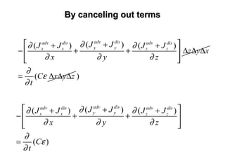
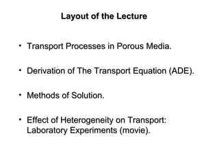
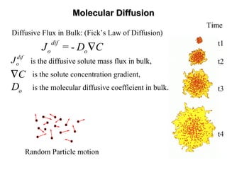
26. General Form of The Transport EquationGeneral Form of The Transport Equation
[ ]
}
}
/
( ')
Dispersion Diffusion
Advection Source SinkChemical reaction
Decay
ij i
i j i
C C S C C W
v C + Q CD
t x x x
λ
ε ε
−
−
 ∂ ∂ ∂ ∂ −
= − − + 
∂ ∂ ∂ ∂  
6447448 64748 64748
where
C is the concentration field at time t,
Dij
is the hydrodynamic dispersion tensor,
Q is the volumetric flow rate per unit volume of the source or sink,
S is solute concentration of species in the source or sink fluid,
i, j are counters,
C’ is the concentration of the dissolved solutes in a source or sink,
W is a general term for source or sink and
vi
is the component of the Eulerian interstitial velocity in xi
direction
defined as follows,
ij
i
j
K
= -v
xε
∂Φ
∂
where
Kij
is the hydraulic conductivity tensor, and ε is the porosity of the medium.

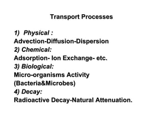
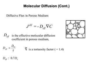
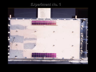
27. Schematic Description of ProcessesSchematic Description of Processes
Figure 7. Schematic Description of the Effects of Advection, Dispersion, Adsorption, and Degradation on Pollution
Transport [after Kinzelbach, 1986].
Advection+Dispersion
Advection
Advection+Dispersion+Adsorption
Advection+Dispersion+Adsorption+Degradation

28. Methods of SolutionMethods of Solution
1) Analytical Approaches:1) Analytical Approaches:
2) Numerical Approaches:2) Numerical Approaches:
i)i) Eulerian Methods:(FDM,FEM).Eulerian Methods:(FDM,FEM).
ii) Lagrangian Methods:(RWM).ii) Lagrangian Methods:(RWM).
iii) Eulerian-Lagrangian Methods:iii) Eulerian-Lagrangian Methods:
(MOC).(MOC).

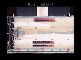
29. Pulse versus Continuous InjectionPulse versus Continuous Injection
Concentration Distribution in case of Pulse and Continuous Injections in a 2D Field
[after Kinzelbach, 1986].






tV4
)Y-(y
+
tV4
)tV-X-(x
-
tV4tV4
H)/(M
=t)y,C(x,
xt
2
o
xl
2
xo
xtxl
o
αααπαπ
ε
exp ( )
d
tV4
Y-y
+
tV4
tV-X-x
-
tV4
HM=ty,x,C
t
xt
2
o
xl
2
xo
tlx
o
∫ 





−−
−
−
•
0
)(
)(
)(
)((
exp
1)(/
)( τ
τατα
τ
τααπ
ε

30. Flow
t = 0
f
t = Flowing Time
Var(X)
The spread of the front is a measure of the heterogeneity
Random WalkRandom Walk

31. Analytical versus Random WalkAnalytical versus Random Walk

32. Scale dependent dispersivityScale dependent dispersivity

33. Experimental Set upExperimental Set up

34. Experiment No. 1Experiment No. 1

35. Experiment No. 2Experiment No. 2