This document provides an overview of control systems and introduces key concepts that will be covered in the course. It discusses: 1) The class of systems that will be studied are single-input single-output, linear, time-invariant, causal dynamic systems modeled by ordinary differential equations with constant coefficients. 2) Control systems can be open-loop or closed-loop. Closed-loop systems use feedback to make them more robust to disturbances. This course will focus on closed-loop feedback control. 3) A basic example of a closed-loop control system is presented using a DC motor, with the goal of maintaining a desired output speed despite disturbances or changes. Feedback is used to calculate the error between

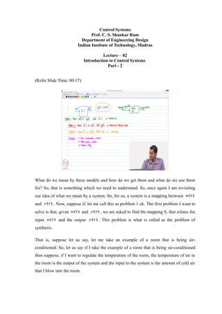
1. Control Systems
Prof. C. S. Shankar Ram
Department of Engineering Design
Indian Institute of Technology, Madras
Lecture – 02
Introduction to Control Systems
Part - 2
(Refer Slide Time: 00:17)
What do we mean by these models and how do we get them and what do we use them
for? So, that is something which we need to understand. So, once again I am revisiting
our idea of what we mean by a system. So, for us, a system is a mapping between )(tu
and )(ty . Now, suppose if, let me call this as problem 1 ok. The first problem I want to
solve is that, given )(tu and )(ty , we are asked to find the mapping S, that relates the
input )(tu and the output )(ty . This problem is what is called as the problem of
synthesis.
That is, suppose let us say, let me take an example of a room that is being air-
conditioned. So, let us say if I take the example of a room that is being air-conditioned
then suppose, if I want to regulate the temperature of the room, the temperature of air in
the room is the output of the system and the input to the system is the amount of cold air
that I blow into the room.

2. Let us say we have a room air conditioner and let us say the temperature of air in the
room is my output and let us say the amount of cold air provided right to the room
through the ac vents is the input of the system. So, what would this synthesis problem
entail? The problem of synthesis essentially means that I provide varying quantities of
the input to the system and then measure the output and try to get a mapping between the
two. So, that is what I do so that I get a mathematical model for the system.
So, in this case, if I provide various amounts of cold air to my air conditioner and I
measure the corresponding temperature and I get a relationship between the two, then I
will know how the temperature of air in this particular room would vary. So, once I do
this first problem of synthesis, I can go and do problem number 2, which is going to be
the following: Given the mapping S, once we find the mapping S, and given a particular
input )(tu , find )(ty .
Suppose, I have got a mathematical model for the temperature of air in this room
equipped with an air conditioner. So, tomorrow let us say, I want to essentially change
the air conditioner and let us say I have 5 choices. Without even purchasing them I can
use the model which I have developed to figure out how temperature would vary and
settle down to a desired value by doing this analysis right, once I have the mathematical
model for this particular process of air conditioning.
So, the advantage is that I can predict the temperature variation without even buying the
air conditioner, installing it and testing it so that I can make a well-informed choice as far
as which AC to buy. So, this problem is what is called the analysis problem or the
prediction problem.
Another problem, which we can do once we complete the synthesis problem is that,
given the mapping S and a desired output )(ty , find )(tu . That is the third problem
that we can solve. So, this problem is what is called the control problem.
So, what do I mean by this? Suppose, let us say I come into a room with an air
conditioner and I essentially want to regulate the temperature of air in this room. So, I set
the temperature of the air at 25 degree Celsius. The question is that, what is the amount
of cold air, which I should blow, which would get my temperature to 25 degree Celsius.
That is the problem of control.

3. So, I know what the mapping of the dynamic system is and I want the desired output,
what is the input which I have to provide? So, in a certain sense, it is the inverse problem
of what we do in problem number 2. So, this mapping helps us to find a )(ty given a
)(tu . In the problem of control, what we do is that, given )(ty I want to use this
mapping to find what )(tu will get me the output )(ty . So, that is the problem of
control.
So, what are a few examples of control that we have already look at? One is room
temperature control. So, that is, that is one example that we have discussed. Let us say,
we have also looked at an example, where we want to control the speed of a motor. And
our human body is a marvellous controller.
Say, for example, our human body maintains our body temperature in a very-very narrow
band. So, even if the temperature goes to 100 degrees Fahrenheit right, so we are in
trouble, correct. So, essentially our body maintains our internal body temperature, in a
very narrow band irrespective of what that environment temperature is.
So, it does not matter whether we are in winter or in summer you know the human
internal body temperature is maintained at almost a constant value and that is a great
control system. For example, the blood pressure that is maintained by your body. You
know it should be in a good range. Blood sugar level is another marvellous control
mechanism. And in fact, even our heart which is a pump which essentially pumps blood
throughout the body needs to work repeatedly again and again as far as we live. So, that
is extremely important to us. So, our human body is filled with marvellous controllers,
which regulate various variables around the desired values very accurately and for a long
time and that is something which is marvellous.
So, essentially we are going to look at various case studies, as we go along and then we
will see how to formulate practical problems as a control problem and solve them, ok.
So, before we get into the mathematics I just want to give another physical perspective,
as far as how we look at control and so on.

4. (Refer Slide Time: 08:41)
So, essentially in a very broad sense, people classify control as what is called an open
loop control and closed loop control. What are these terms? Let us say we consider the
example of a ceiling fan. So, I have a ceiling fan, I have a regulator and I have a switch,
right. I can come, switch on the fan and I can vary the speed setting, maybe in discrete
quantities by using the fan speed regulator and that is about it, right.
So, I just get some output, which is a fan RPM. So, that is an open loop controller in the
sense that, it cannot account for any disturbances, which come during the operation of
the fan. For example, if there is a voltage fluctuation, then, the output of the fan or the
speed of rotation of the fan is going to fall down or go up depending on whether the
voltage is falling down or going up. So, then, you know like, the question is that like I
lose certain performance right, but the question we need to ask ourselves is that, is it
important, for a ceiling fan? So, typically ceiling fans are open loop control systems,
where the speed settings are calibrated in the factory and the regulator essentially, adjusts
the fan RPM in a discrete set of values.
Essentially in the presence of disturbances, obviously, the system response gets affected.
So, that is the characteristic of open-loop control. So, what are the various characteristics
of open loop control: There is no feedback (we will shortly define what is called as
feedback). So, essentially, it cannot tolerate disturbances; it is not robust to disturbances
and so on, ok. But on the flip side, the cost and complexity are lower.

5. On the other hand, if we want a fan, whose RPM needs to be maintained at a baseline
value, let us say 100 RPM and I cannot afford a huge variation in the RPM, right, for
some industrial application, what would I do? What I would do is that, I would measure
the actual RPM using a speed sensor and then I would take the actual RPM at each and
every instant of time, compare it with what is the desired value and then take the
difference, quantify the difference between what I desire and what is actually being
obtained, take that error and pass it through what is called as a controller and the
controller will then adjust the electrical input to the fan. Then, when that happens we
have what is called as closed-loop control and closed loop control systems have
feedback. Feedback is the process of measuring variables that need to be regulated or
controlled so that corrective action can be taken ok, that is the process of feedback.
So, consequently closed loop control is more tolerant or robust to uncertainties that come
in disturbances and so on (what we call as un-modelled dynamics). So, but anyway let
me group them under uncertainties, ok. But the flipside of closed-loop control is that the
cost and complexity are higher.
In this particular course, we are going to deal with closed-loop control. So, that is what
we are going to deal with in this particular course. So, let me just construct an example to
just explain what we did. Suppose, let us say, we have, let us say, a DC motor right. So,
the DC motor is our system or plant, ok. And to this DC motor, let us say, I provide a
voltage )(tV as my input and )(t is my output.
Suppose, let us say I want a desired output (desired RPM of rotation from the motor) and
this is what we call as a reference input and what we do then is the following. Suppose if
I measure the actual output, then what I do is that I go and compare, then I take the
difference between what I desire and what I measure, which is what is called as the error
and then, let us say, we pass it through an element called as a controller and the
controller then calculates what should be the input that should be provided to the DC
motor, ok.
When the controller calculates the input that should be provided to the system, the
adjective control is added to the term ‘input’. So, the input to the system becomes what is
called as the control input. So, this is feedback, ok. So, this is a typical layout of a closed
loop control system with what is called as negative feedback, ok.

6. So, this is essentially closed loop control system with negative feedback. Why is it
negative feedback? Because at the summing junction you can see that, we are subtracting
the feedback signal from the desired reference input. So, that is why it is called as
negative feedback.
So, we are taking the difference between the reference input and the actual output and
calculating the error. This is what is called a closed loop control system with negative
feedback. So, we can see that this is what we are going to essentially do in this particular
course. So, some more terms that I want to introduce here is that, like, this process of
essentially taking this output measurement and feeding it back is what is called as
feedback. This is what is called a feedback path.
(Refer Slide Time: 17:47)
Typically, we can have a mapping in the feedback path, say we can have some sensor
dynamics coming into play here. So, let us say I use a sensor for measuring speed, the
sensor may have its own dynamic characteristics. I may need to use a filter to filter out
noise, then a mapping comes in the feedback path ok.
So, if a mapping comes in the feedback path (when the mapping is not one ) we call it as
a non-unity feedback. So, when this mapping in the feedback path is 1, we call it as unity
feedback. We will see how this affects our analysis later on right and many times when
the controller calculates and provides a control signal to the system, it is typically
realized by what is called an actuator.

7. Say, for example, let us say you know I have to essentially move, say, design a motion
control system that essentially displaces a work piece along one axis right. Let us say,
simple translation of a work piece in a machining system. So, let us say, I want to
regulate the position of the work piece. I give a, a voltage signal to, let us say, an electric
motor drive system, which essentially provides translational motion to the work piece
right. Suppose, if the controller calculates that, at this point of time, provide 5 volts of
input right to the electric motor or if it calculates and tells me that look, you know like,
provide, you know like, 10 Newton’s of force to the work piece, in order to essentially
move by some distance x , right. So, the controller may say, provide 10 Newton’s at this
instant of time, but then there may be a small, what to say, response time before the 10
Newton’s is actually realized in practice through the electric motor and drive system,
right.
So, that, if that is important then you know, we need to figure out what is called as
actuator dynamics in the design process, ok and sometimes we can have disturbances
coming into the system. Let us say, I have a sudden load that may come on a DC motor,
right, for example, you know that I mean to model as a disturbance and then like see how
we can overcome such disturbances and so on, right.
So, one can see that, you know, we can add varying levels of complexity to this,
feedback system, ok. We are going to study the basic feedback loop in this particular
course and as we go along maybe when we go to some case studies, we will add some
more blocks and then see how the design varies.
To summarize, what we are going to do in this course is the following. So, as a summary
of all this discussion that we did, the title of our course is control systems, right. So, what
we are going to do, what we are going to learn is the following: Closed Loop Feedback
Control of SISO LTI Causal Dynamic Systems. So, that is what we are going to do in
this particular course, ok.
So, that is the class of systems that we are going to do, SISO LTI causal dynamic system
and we are going to do what is called as closed loop feedback control, right, of this class
of systems and it so turns out that this class of systems, SISO LTI causal dynamic
systems, the mathematical models that are typically used to characterize this class of

8. systems usually take the form of a Linear Ordinary Differential Equations, what are
abbreviated as ODEs, with constant coefficients.
So, typically the mathematical models that are used to characterize this class of systems
that we are going to study in this particular course take the form of linear ordinary
differential equations with constant coefficients, ok. So, that is the class of equations that
we would be focusing on.
And, another important aspect is that the kind of mathematical models we are going to
essentially look at are what are called as spatially homogeneous. That means that we do
not consider the variations of variables with space. So, we only consider temporal
variations of variables. For example, let us say, I want to analyze the variation of the
temperature of air in this room, right. So obviously, the temperature of the air in this
room can be different depending on the point where I am measuring and also the time at
which I measure, right. So, but then what we do is that we lump all the points in this
room i.e. the temperature of all the points in this room into a single entity, which
essentially can be represented as a function of time, ok.
So, in a certain sense, what we are doing is that we are lumping the effects as far as
spatial variation is concerned and we are going to assume that the entire room can be
characterized by a single temperature which is only a function of time, ok. So, spatially
homogeneous means we are essentially following sort of a lumped parameter approach
towards our modelling.
Then we are going to have what are called continuous time, dynamic, deterministic,
mathematical models, ok. That is the class of models we are going to use, right. So,
essentially in a certain sense, continuous time means that we treat time as a continuous
variable. So from a pragmatic perspective, it just means that we are going to get ODEs
right, Ordinary Differential Equations. Dynamic means we are going to have derivatives
in the equations.
So, what is a dynamic model? It is something which explicitly considers future states of
the system, right, so, and it essentially incorporates what is going to happen to the system
in the future by incorporating derivatives of the variables. So, that is a dynamic model.
Deterministic means we essentially neglect any stochastic effects, ok. We do not consider

9. variables as random variables. We consider all variables as deterministic variables and
we are going to have deterministic models, ok.
So, this is the class of models that we are going to use. So, in summary, what we are
going to do in this course is closed loop feedback control of SISO LTI causal dynamic
systems using spatially homogeneous, continuous time, dynamic, deterministic
mathematical models, ok. So, that is what we are going to essentially learn how to do in
this course, ok. So, what we would subsequently do is essentially have a brief recap of
what is the mathematical background that is required to do this analysis, ok.
So, that is something which we are going to recap. It is assumed that some mathematical
courses have already been completed before one comes to this particular course,
particularly courses on complex variables, ordinary differential equations and Laplace
transform. So, we would quickly recap some of these tools and then we will move
forward, ok. So, that is going to be the plan of action. Fine.
Thank you.