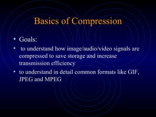
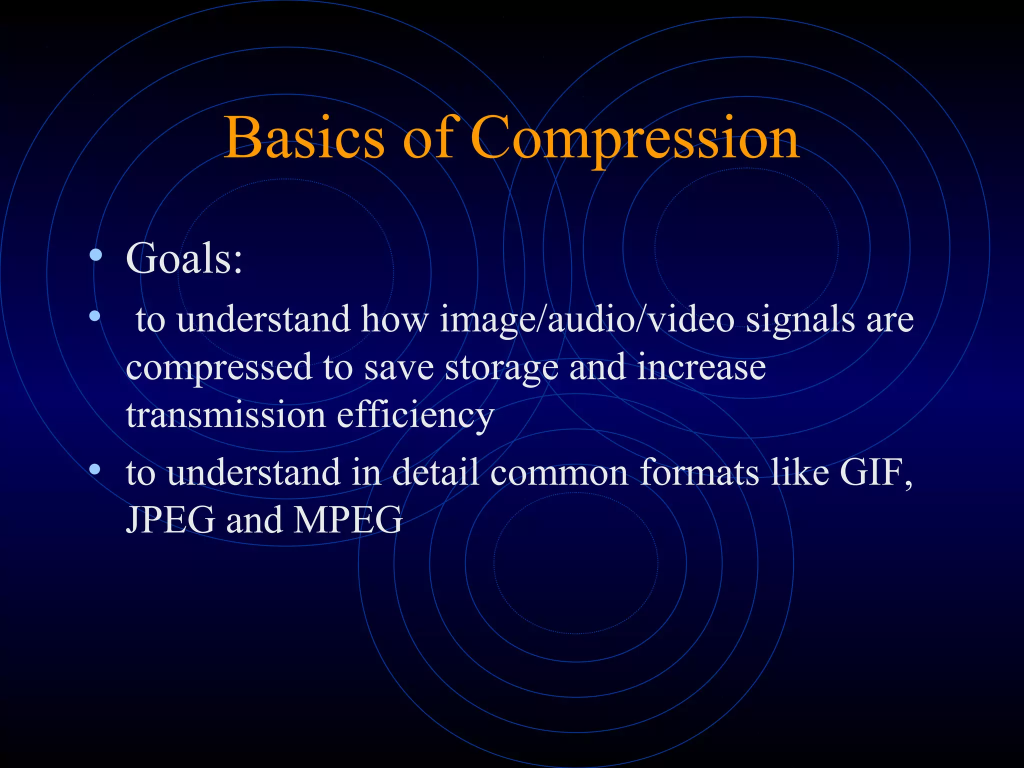
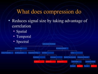
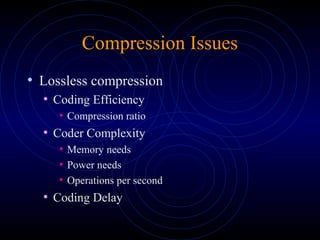
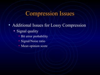
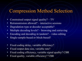
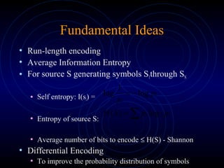
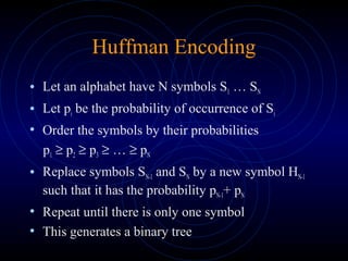
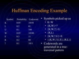
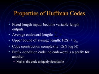
This document discusses various methods of data compression. It begins by stating the goals of understanding how media such as images, audio and video are compressed to reduce file sizes and increase transmission efficiency. It then describes different types of correlations exploited in compression, such as spatial, temporal and spectral. The remainder of the document details specific compression techniques including Huffman coding, Golomb-Rice coding, and lossless JPEG. It discusses considerations for compression method selection such as output quality, encoding/decoding delay, and whether lossy or lossless compression is required.

1. Basics of Compression
• Goals:
• to understand how image/audio/video signals are
compressed to save storage and increase
transmission efficiency
• to understand in detail common formats like GIF,
JPEG and MPEG

2. What does compression do
• Reduces signal size by taking advantage of
correlation
• Spatial
• Temporal
• Spectral
L in e a r P r e d ic t iv e A u t o R e g r e s s iv e P o ly n o m ia l F it t in g
M o d e l- B a s e d
H u ffm a n
S t a t is t ic a l
A r it h m e t ic L e m p e l- Z iv
U n iv e r s a l
L o s s le s s
S p a t ia l/ T im e - D o m a in
S u b b a n d W a v e le t
F ilt e r - B a s e d
F o u r ie r D C T
T r a n s fo r m - B a s e d
F r e q u e n c y - D o m a in
L o s s y
W a v e fo r m - B a s e d
C o m p r e s s io n M e t h o d s

3. Compression Issues
• Lossless compression
• Coding Efficiency
• Compression ratio
• Coder Complexity
• Memory needs
• Power needs
• Operations per second
• Coding Delay

4. Compression Issues
• Additional Issues for Lossy Compression
• Signal quality
• Bit error probability
• Signal/Noise ratio
• Mean opinion score

5. Compression Method Selection
• Constrained output signal quality? – TV
• Retransmission allowed? – interactive sessions
• Degradation type at decoder acceptable?
• Multiple decoding levels? – browsing and retrieving
• Encoding and decoding in tandem? – video editing
• Single-sample-based or block-based?
• Fixed coding delay, variable efficiency?
• Fixed output data size, variable rate?
• Fixed coding efficiency, variable signal quality? CBR
• Fixed quality, variable efficiency? VBR

6. Fundamental Ideas
• Run-length encoding
• Average Information Entropy
• For source S generating symbols S1through SN
• Self entropy: I(si) =
• Entropy of source S:
• Average number of bits to encode ≤ H(S) - Shannon
• Differential Encoding
• To improve the probability distribution of symbols
i
i
p
p
log
1
log −=
∑=
i
ii ppSH 2log)(

7. Huffman Encoding
• Let an alphabet have N symbols S1 … SN
• Let pi be the probability of occurrence of Si
• Order the symbols by their probabilities
p1 ≥ p2 ≥ p3 ≥ … ≥ pN
• Replace symbols SN-1 and SN by a new symbol HN-1
such that it has the probability pN-1+ pN
• Repeat until there is only one symbol
• This generates a binary tree

8. Huffman Encoding Example
• Symbols picked up as
• K+W
• {K,W}+?
• {K,W,?}+U
• {R,L}
• {K,W,?,U}+E
• {{K,W,?,U,E},{R,L}}
• Codewords are
generated in a tree-
traversal pattern
Symbol Probability Codeword
K 0.05 10101
L 0.2 01
U 0.1 100
W 0.05 10100
E 0.3 11
R 0.2 00
? 0.1 1011

9. Properties of Huffman Codes
• Fixed-length inputs become variable-length
outputs
• Average codeword length:
• Upper bound of average length: H(S) + pmax
• Code construction complexity: O(N log N)
• Prefix-condition code: no codeword is a prefix for
another
• Makes the code uniquely decodable
∑ iipl

10. Huffman Decoding
• Look-up table-based decoding
• Create a look-up table
• Let L be the longest codeword
• Let ci be the codeword corresponding to symbol si
• If ci has li bits, make an L-bit address such that the first li bits
are ci and the rest can be any combination of 0s and 1s.
• Make 2^(L-li) such addresses for each symbol
• At each entry, record, (si, li) pairs
• Decoding
• Read L bits in a buffer
• Get symbol sk, that has a length of lk
• Discard lk bits and fill up the L-bit buffer

11. Constraining Code Length
• The problem: the code length should be at most L bits
• Algorithm
• Let threshold T=2-L
• Partition S into subsets S1 and S2
• S1= {si|pi > T} … t-1 symbols
• S2= {si|pi ≤ T} … N-t+1 symbols
• Create special symbol Q whose frequency q =
• Create code word cq for symbol Q and normal
Huffman code for every other symbol in S1
• For any message string in S1, create regular code word
• For any message string in S2, first emit cq and then a regular
code for the number of symbols in S2
∑=
N
ti
ip

12. Constraining Code Length
• Another algorithm
• Set threshold t like before
• If for any symbol si, pi ≤ T, set pi = T
• Design the codebook
• If the resulting codebook violates the ordering of code
length according to symbol frequency, reorder the
codes
• How does this differ from the previous algorithm?
• What is its complexity?

13. Golomb-Rice Compression
• Take a source having symbols occurring with a geometric
probability distribution
• P(n)=(1-p0) pn
0 n≥0, 0<p0<1
• Here is P(n) the probability of run-length of n for any symbol
• Take a positive integer m and determine q, r where
n=mq+r.
• Gm code for n: 0…01 + bin(r)
• Optimal if
• m =
q has log2m bits if
r >sup(log2m)





 +
−
)log(
)1log(
0
0
p
p

14. Golomb-Rice Compression
• Now if m=2k
• Get q by k-bit right shift and r by last r bits of n
• Example:
• If m=4 and n=22 the code is 00000110
• Decoding G-R code:
• Count the number of 0s before the first 1. This gives q.
Skip the 1. The next k bits gives r

15. The Lossless JPEG standard
• Try to predict the value of pixel X as
prediction residual r=y-X
• y can be one of 0, a, b, c, a+b-c, a+(b-c)/2,b+
(a-c)/2
• The scan header records the choice of y
• Residual r is computed modulo 216
• The number of bits needed for r is called its
category, the binary value of r is its
magnitude
• The category is Huffman encoded
c b
a X