Download as PDF, PPTX

![LDA: Inference
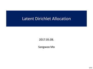
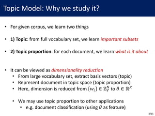
• Recall:
• Find MAP assignment of latent variables
𝑝 𝛽, 𝜃, 𝑧 𝑤, 𝛼, 𝜂 =
𝑝(𝛽, 𝜃, 𝑧, 𝑤|𝛼, 𝜂)
∫ ∫ ∑ 𝑝(𝛽, 𝜃, 𝑧, 𝑤|𝛼, 𝜂)[]
• Posterior is intractable; We use techniques e.g. MCMC, VI, etc.
• Today, I will only introduce variational inference
8/15](https://image.slidesharecdn.com/lda-170508042034/85/Latent-Dirichlet-Allocation-8-320.jpg)
![LDA: Variational Inference
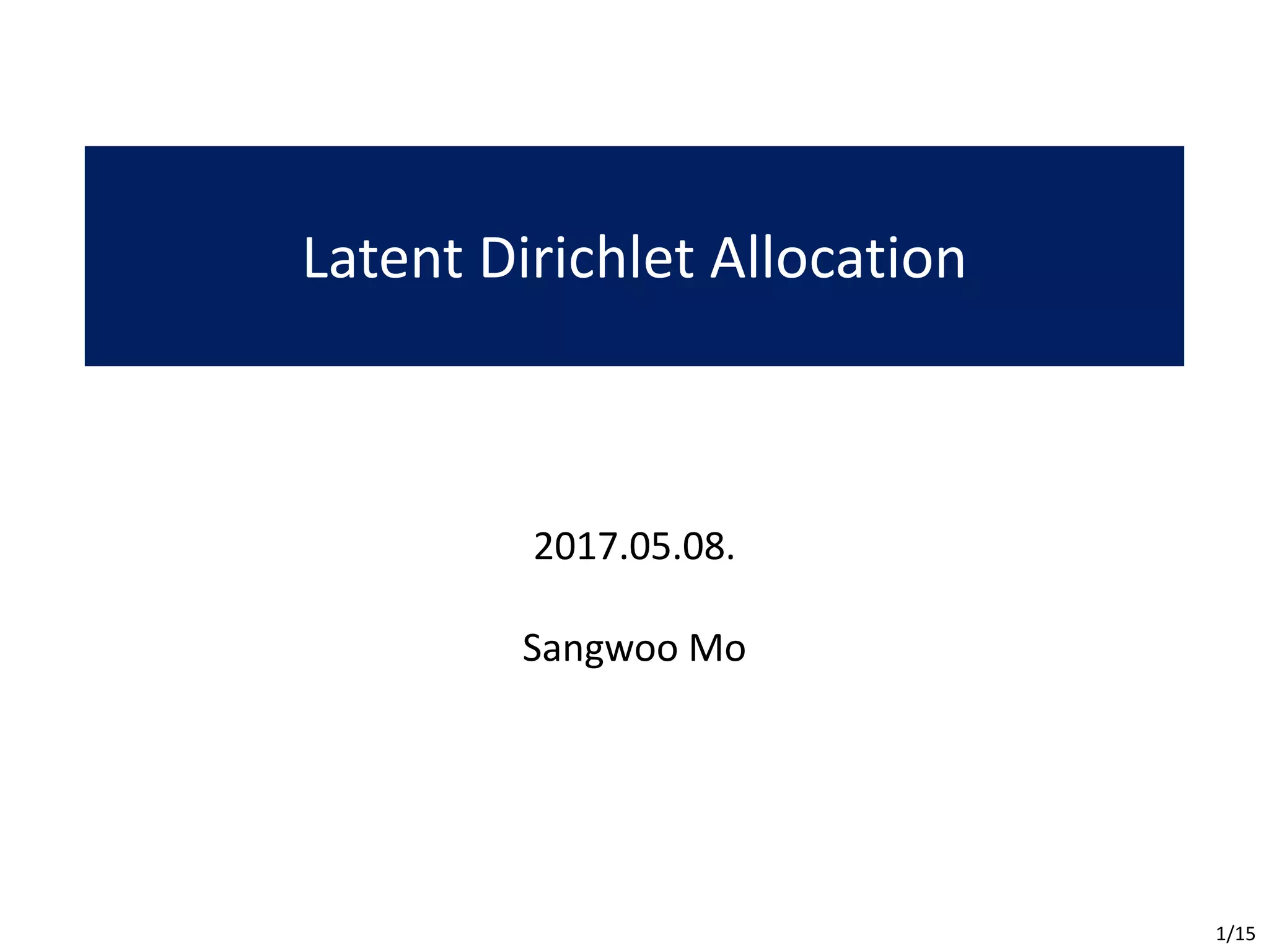
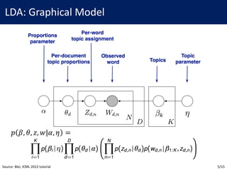
• Approximate 𝑝(𝛽, 𝜃, 𝑧|𝑤, 𝛼, 𝜂) with 𝑞(𝛽, 𝜃, 𝑧|𝜆, 𝛾, 𝜑) where
𝑞 𝛽, 𝜃, 𝑧 𝜆, 𝛾, 𝜑 = ∏𝑞 𝛽< 𝜆< ∏ 𝑞 𝜃B 𝛾B ∏𝑞 𝑧B,E 𝜑B,E
• Goal: Minimize 𝐾𝐿(𝑞||𝑝) over (𝜆, 𝛾, 𝜑)
• However, 𝐾𝐿(𝑞||𝑝) is intractable since
𝑝 𝛽, 𝜃, 𝑧 𝑤, 𝛼, 𝜂 =
𝑝(𝛽, 𝜃, 𝑧, 𝑤|𝛼, 𝜂)
∫ ∫ ∑ 𝑝(𝛽, 𝜃, 𝑧, 𝑤|𝛼, 𝜂)[]
is intractable; Thus, we optimize alternative objective
10/15](https://image.slidesharecdn.com/lda-170508042034/85/Latent-Dirichlet-Allocation-10-320.jpg)
![LDA: Variational Inference
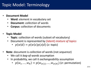
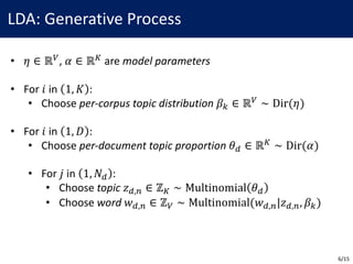
• Recall: Want to minimize 𝐾𝐿(𝑞||𝑝), but it is intractable
• Alternative Goal: Maximize ELBO 𝐿 𝜆, 𝛾, 𝜑; 𝛼, 𝜂 where
𝐿 𝜆, 𝛾, 𝜑; 𝛼, 𝜂 = 𝐸f log 𝑝 𝛽, 𝜃, 𝑧, 𝑤 𝛼, 𝜂 − 𝐸f[log 𝑞(𝛽, 𝜃, 𝑧|𝛼, 𝜂)]
• Since log 𝑝(𝑤|𝛼, 𝜂) = 𝐿 𝜆, 𝛾, 𝜑; 𝛼, 𝜂 + 𝐾𝐿(𝑞||𝑝),
minimizing 𝐾𝐿(𝑞||𝑝) is equal to maximizing 𝐿 𝜆, 𝛾, 𝜑; 𝛼, 𝜂
11/15](https://image.slidesharecdn.com/lda-170508042034/85/Latent-Dirichlet-Allocation-11-320.jpg)
![LDA: Variational Inference
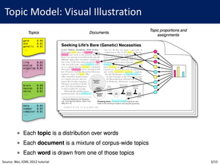
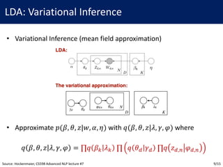
• Maximize ELBO 𝐿 𝜆, 𝛾, 𝜑; 𝛼, 𝜂 where
𝐿 𝜆, 𝛾, 𝜑; 𝛼, 𝜂 = 𝐸f log 𝑝 𝛽, 𝜃, 𝑧, 𝑤 𝛼, 𝜂 − 𝐸f[log 𝑞(𝛽, 𝜃, 𝑧|𝛼, 𝜂)]
• Final Goal: maximize 𝐿 𝜆, 𝛾, 𝜑; 𝛼, 𝜂 over 𝜆, 𝛾, 𝜑, 𝛼, 𝜂
• Idea: divide hard problem into two (relatively) easy problems
• 1) maximize 𝐿 𝜆, 𝛾, 𝜑, 𝛼, 𝜂 over 𝜆, 𝛾, 𝜑
• 2) maximize 𝐿 𝜆, 𝛾, 𝜑, 𝛼, 𝜂 over (𝛼, 𝜂)
Source: Hockenmaier, CS598 Advanced NLP lecture #7 12/15](https://image.slidesharecdn.com/lda-170508042034/85/Latent-Dirichlet-Allocation-12-320.jpg)
![LDA: Variational EM
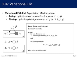
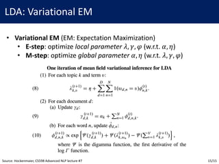
• Variational EM (EM: Expectation Maximization)
• E-step: optimize local parameter 𝜆, 𝛾, 𝜑 (w.r.t. 𝛼, 𝜂)
• M-step: optimize global parameter 𝛼, 𝜂 (w.r.t. 𝜆, 𝛾, 𝜑)
• Each subproblem is simple one-variable constraint optimization
• We can solve it by taking derivative of Lagrangian to zero1
• e.g. optimize 𝐿 over 𝜑 (since 𝜑 ∼ Multinomial, ∑ 𝜑E/
5
/P) = 1)
1. In fact, 𝐿[l] cannot be solved analytically. Authors suggest to use Netwon-Raphson method for efficient implementation.
See A.3 and A.4 of Blei 2003 for detail.
Source: Blei, JMLR 2003 paper 14/15](https://image.slidesharecdn.com/lda-170508042034/85/Latent-Dirichlet-Allocation-14-320.jpg)
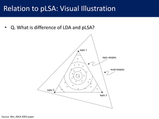

This document provides an overview of Latent Dirichlet Allocation (LDA), a generative probabilistic model for collections of discrete data such as text corpora. It defines key terminology for LDA including documents, words, topics, and distributions. The document then explains LDA's graphical model and generative process, which represents documents as mixtures over latent topics and generates words probabilistically from topics. Variational inference is introduced as an approach for approximating the intractable posterior distribution over topics and learning model parameters.