Reducing the Sampling
Complexity of Topic Models
Aaron Li
joint work with Amr Ahmed, Sujith Ravi, Alex Smola
CMU and Google
Outline
• Topic Models
• Inference algorithms
• Losing sparsity at scale
• Inference algorithm
• Metropolis Hastings proposal
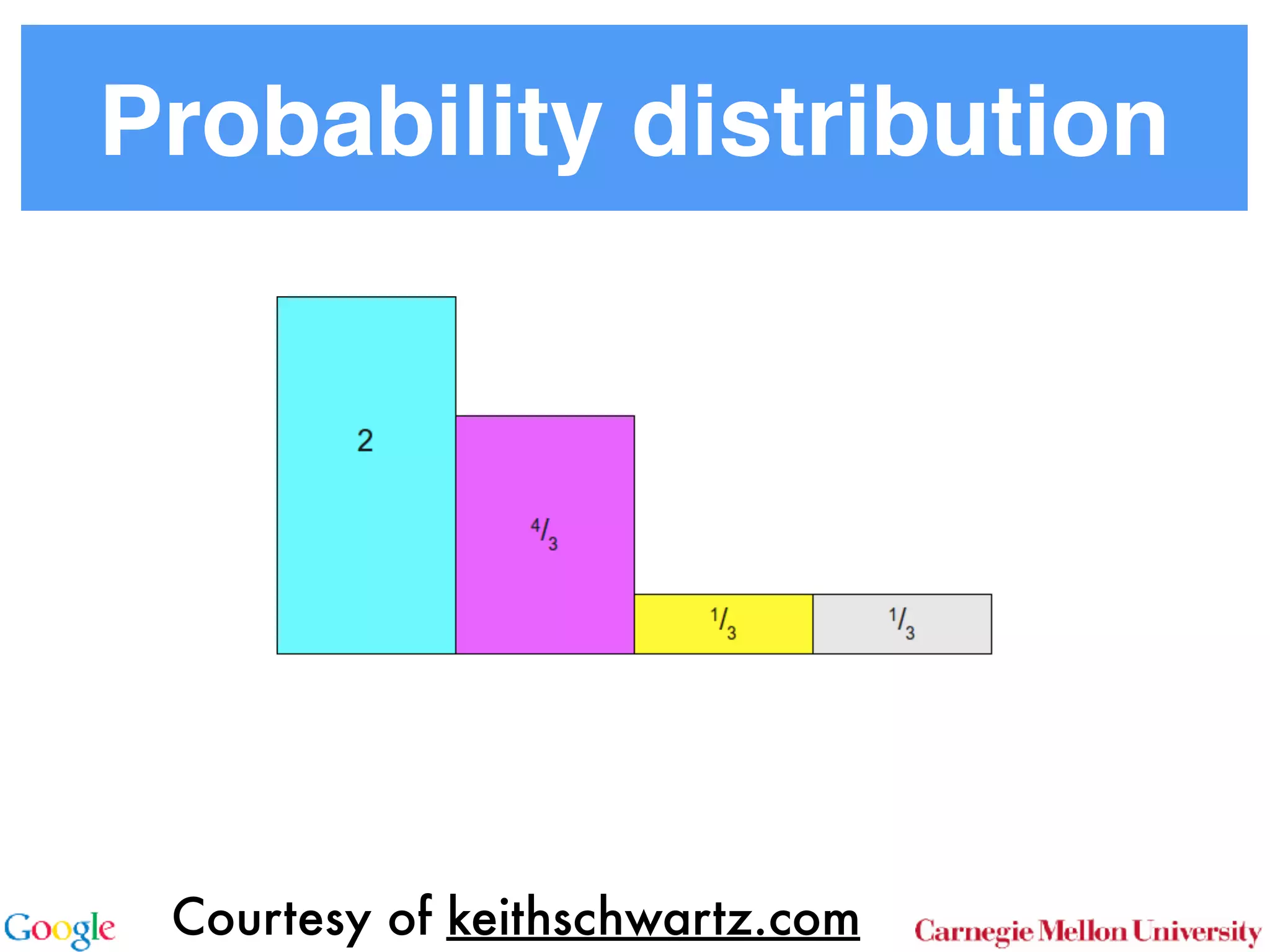
• Walker’s Alias method for O(kd) draws
• Experiments
• LDA, Pitman-Yor topic models, HPYM
• Distributed inference
Models
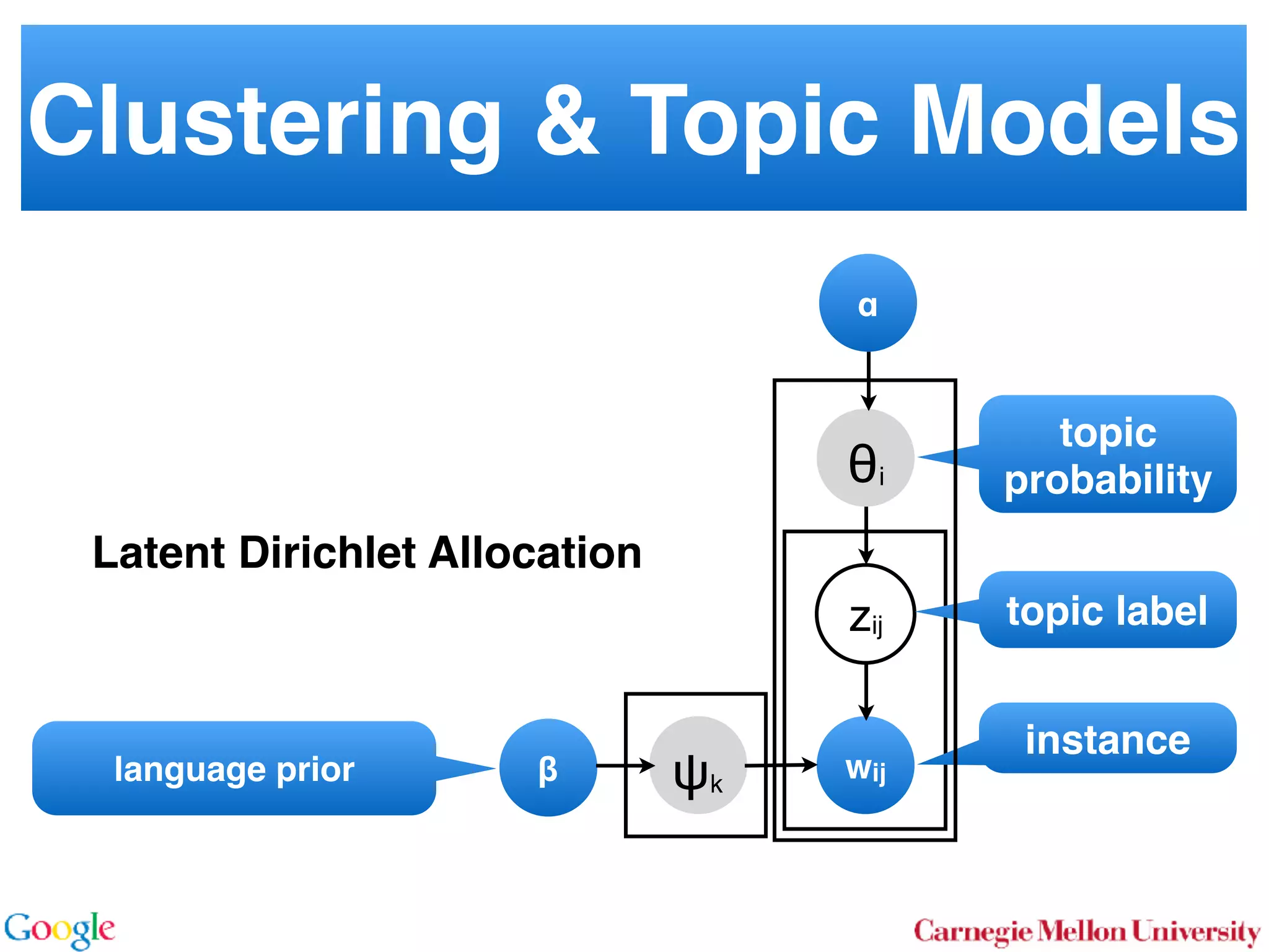
Clustering & Topic Models
Latent Dirichlet Allocation
wij
zij
θi
language prior
topic
probability
topic label
instance
α
β ψk
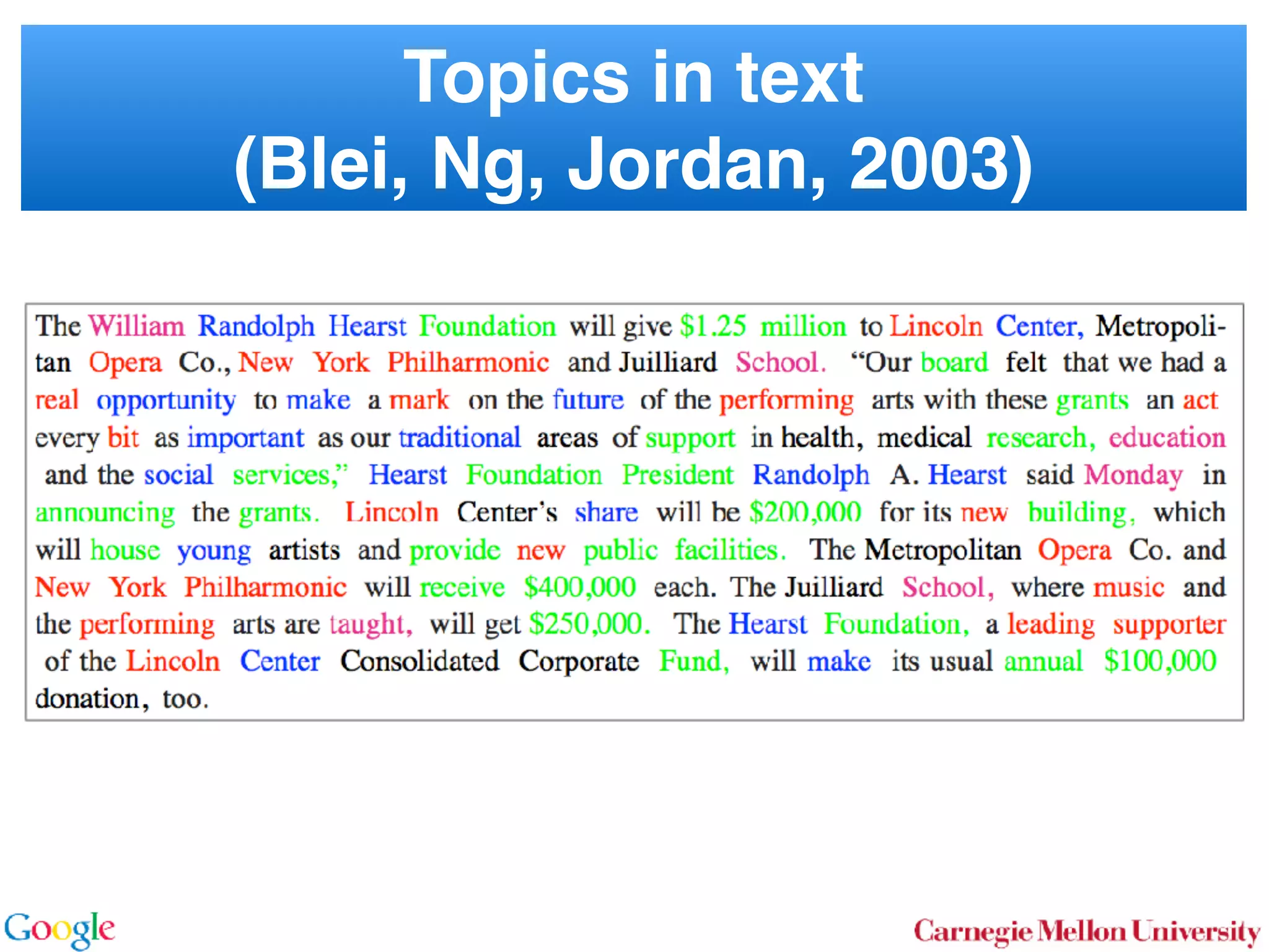
Topics in text

(Blei, Ng, Jordan, 2003)
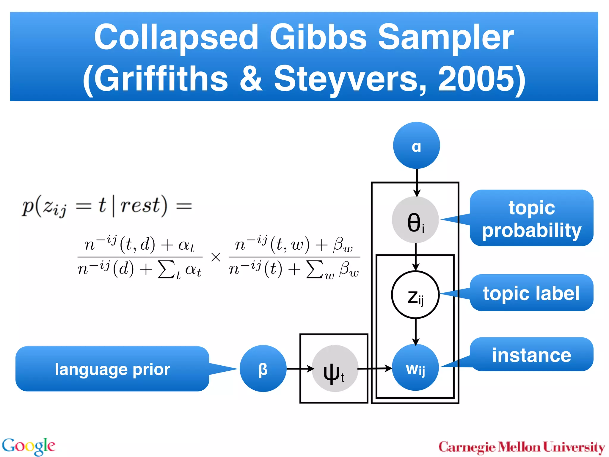
Collapsed Gibbs Sampler

(Griffiths & Steyvers, 2005)
wij
zij
θi
language prior
topic
probability
topic label
instance
α
ψt
β
n ij
(t, d) + ↵t
n ij(d) +
P
t ↵t
⇥
n ij
(t, w) + w
n ij(t) +
P
w w
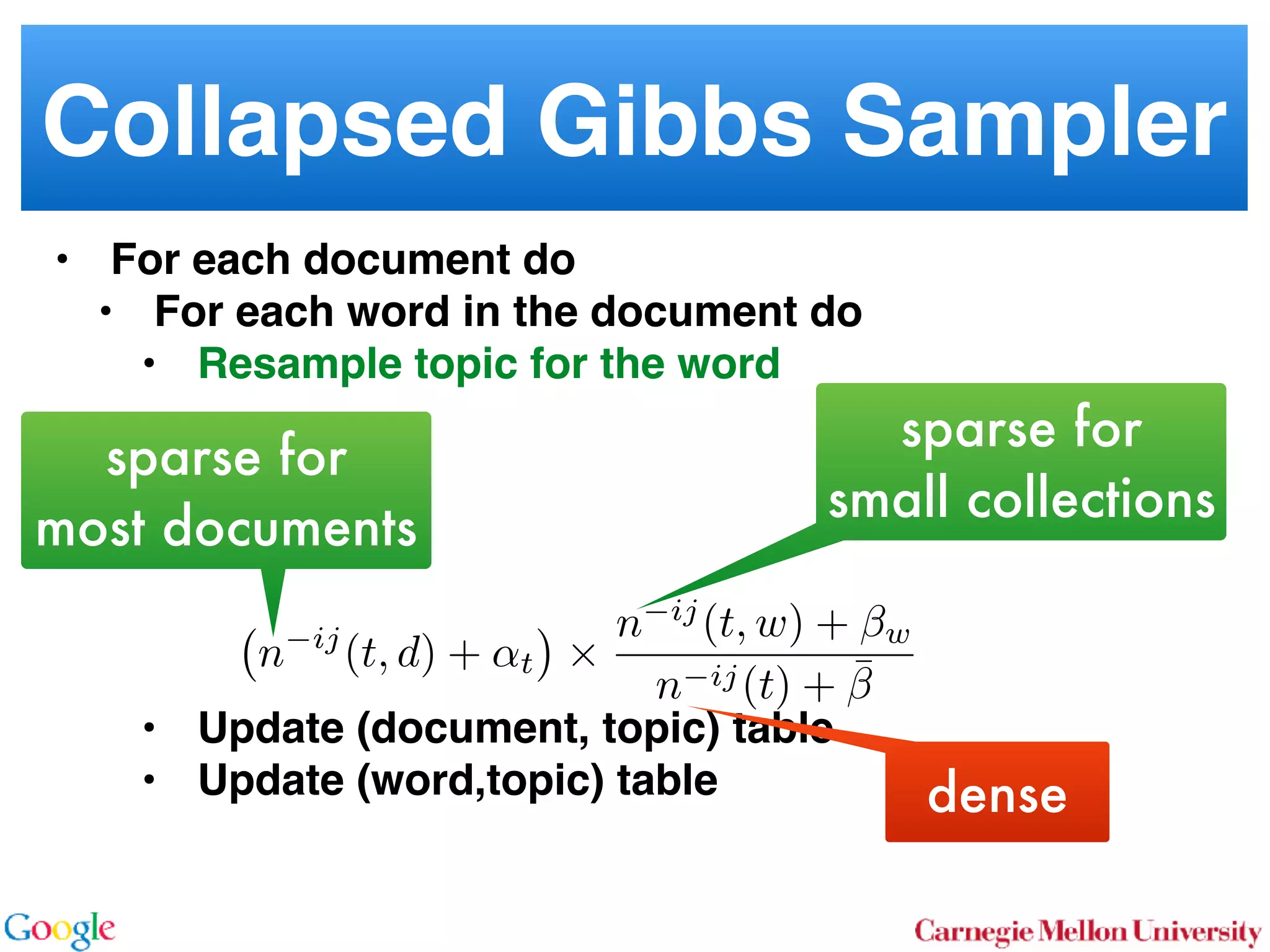
• For each document do
• For each word in the document do
• Resample topic for the word


• Update (document, topic) table
• Update (word,topic) table
Collapsed Gibbs Sampler
sparse for
small collections
sparse for
most documents
dense
n ij
(t, d) + ↵t ⇥
n ij
(t, w) + w
n ij(t) + ¯
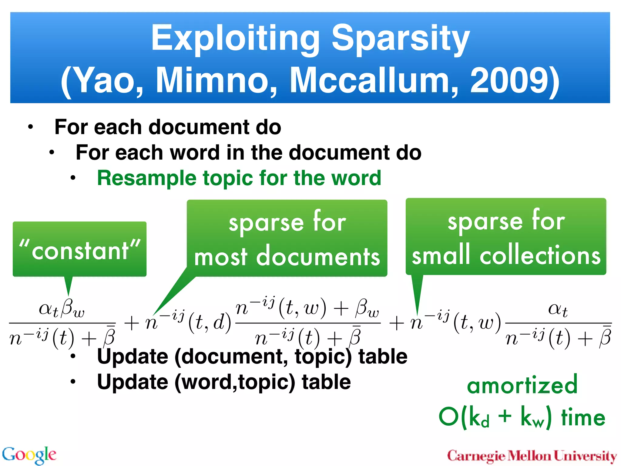
• For each document do
• For each word in the document do
• Resample topic for the word


• Update (document, topic) table
• Update (word,topic) table
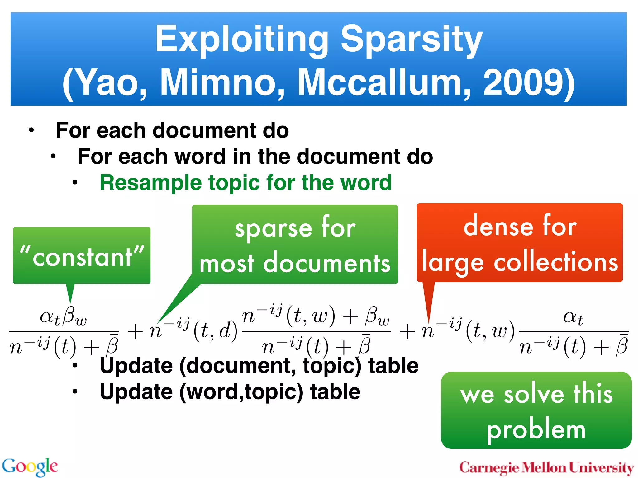
Exploiting Sparsity

(Yao, Mimno, Mccallum, 2009)
sparse for
small collections“constant”
↵t w
n ij(t) + ¯ + n ij
(t, d)
n ij
(t, w) + w
n ij(t) + ¯ + n ij
(t, w)
↵t
n ij(t) + ¯
sparse for
most documents
amortized

O(kd + kw) time
• For each document do
• For each word in the document do
• Resample topic for the word


• Update (document, topic) table
• Update (word,topic) table
Exploiting Sparsity

(Yao, Mimno, Mccallum, 2009)
“constant”
↵t w
n ij(t) + ¯ + n ij
(t, d)
n ij
(t, w) + w
n ij(t) + ¯ + n ij
(t, w)
↵t
n ij(t) + ¯
sparse for
most documents
dense for
large collections
O(k) time
we solve this
problem
More Models
• LDA
• Poisson-Dirichlet Process
2.1 Latent Dirichlet Allocation
In LDA [3] one assumes that documents are mixture dis-
tributions of language models associated with individual
topics. That is, the documents are generated following the
graphical model below:
for all i
for all d
for all k
↵ ✓d zdi wdi k
For each document d draw a topic distribution ✓d from a
Dirichlet distribution with concentration parameter ↵
✓d ⇠ Dir(↵). (1)
For each topic t draw a word distribution from a Dirichlet
distribution with concentration parameter
t ⇠ Dir( ). (2)
For each word i 2 {1 . . . nd} in document d draw a topic
from the multinomial ✓d via
Sto
sampl
using
⌘tw a
Unfor
carefu
dense
Inst
amort
Here
in O(
numb
tional
does n
gle wo
chang
the ba
2.2
To
with m
for all i
for all d
for all k
↵ ✓d zdi wdi t 0
In a conventional topic model the language model is sim-
ply given by a multinomial draw from a Dirichlet distribu-
tion. This fails to exploit distribution information between
topics, such as the fact that all topics have the same common
underlying language. A means for addressing this problem
if n
Her
for
rameter a prevents a word to be sampled too often by im-
posing a penalty on its probability based on its frequency.
The combined model described explicityly in [5]:
✓d ⇠ Dir(↵) 0 ⇠ Dir( )
zdi ⇠ Discrete(✓d) t ⇠ PDP(b, a, 0)
wdi ⇠ Discrete ( zdi )
As can be seen, the document-specific part is identical to
LDA whereas the language model is rather more sophisti-
cated. Likewise, the collapsed inference scheme is analogous
to a Chinese Restaurant Process [6, 5]. The technical di -
culty arises from the fact that we are dealing with distribu-
tions over countable domains. Hence, we need to keep track
of multiplicities, i.e. whether any given token is drawn from
i or 0. This will require the introduction of additional
count variables in the collapsed inference algorithm.
Each topic is equivalent to a restaurant. Each token in the
document is equivalent to a customer. Each type of word
corresponds each type of dish served by the restaurant. The
same results in [6] can be used to derive the conditional
probability by introducing axillary variables:
• stw denotes the number of tables serving dish w in
restaurant t. Here t is the equivalent of a topic.
• rdi indicates whether wdi opens a new table in the
restaurant or not (to deal with multiplicities).
• mtw denotes the number of times dish w has been
served in restaurant t (analogously to nwk in LDA).
The conditional probability is given by:
p(zdi = t, rdi = 0|rest) /
↵t + ndt
bt + mt
mtw + 1 stw
mtw + 1
Smtw+1
stw,at
Smtw
stw,at
(7)
over topics. In other words, we add an extra level o
chy on the document side (compared to the extra h
on the language model used in the PDP).
for all i
for all d
for al
H ✓0 ✓d zdi wdi k
More formally, the joint distribution is as follows:
✓0 ⇠ DP(b0, H(·)) t ⇠ Dir( )
✓d ⇠ DP(b1, ✓0)
zdi ⇠ Discrete(✓d)
wdi ⇠ Discrete ( zdi )
By construction, DP(b0, H(·)) is a Dirichlet Process
lent to a Poisson Dirichlet Process PDP(b0, a, H(·))
discount parameter a set to 0. The base distributio
often assumed to be a uniform distribution in most
At first, a base ✓0 is drawn from DP(b0, H(·)). T
erns how many topics there are in general, and wh
overall prevalence is. The latter is then used in the n
of the hierarchy to draw a document-specific distrib
that serves the same role as in LDA. The main di↵
that unlike in LDA, we use ✓0 to infer which topics
popular than others.
It is also possible to extend the model to more t
levels of hierarchy, such as the infinite mixture mo
Similar to Poisson Dirichlet Process, an equivalent
Restaurant Franchise analogy [6, 19] exists for H
cal Dirichlet Process with multiple levels. In this
each Dirichlet Process is mapped to a single Chinese
for all i
for all d
for all k
d zdi wdi t 0
entional topic model the language model is sim-
y a multinomial draw from a Dirichlet distribu-
if no additional ’table’ is opened by word wdi. Otherwise
p(zdi = t, rdi = 1|rest) (8
/(↵t + ndt)
bt + atst
bt + mt
stw + 1
mtw + 1
+ stw
¯ + st
Smtw+1
stw+1,at
Smtw
stw,at
Here SN
M,a is the generalized Stirling number. It is given b
More Models
• LDA
• Hierarchical-Dirichlet Process


… even more mess for topic distribution
2.1 Latent Dirichlet Allocation
In LDA [3] one assumes that documents are mixture dis-
tributions of language models associated with individual
topics. That is, the documents are generated following the
graphical model below:
for all i
for all d
for all k
↵ ✓d zdi wdi k
For each document d draw a topic distribution ✓d from a
Dirichlet distribution with concentration parameter ↵
✓d ⇠ Dir(↵). (1)
For each topic t draw a word distribution from a Dirichlet
distribution with concentration parameter
t ⇠ Dir( ). (2)
For each word i 2 {1 . . . nd} in document d draw a topic
from the multinomial ✓d via
Sto
sampl
using
⌘tw a
Unfor
carefu
dense
Inst
amort
Here
in O(
numb
tional
does n
gle wo
chang
the ba
2.2
To
with m
pus, the
portional
w from a
ility dis-
mon un-
distribu-
del, each
base dis-
anguage
arameter
le being
ount pa-
n by im-
equency.
0)
ntical to
sophisti-
nalogous
cal di -
distribu-
ep track
twice as large space of state variables.
2.3 Hierarchical Dirichlet Process
To illustrate the e cacy and generality of our approach we
discuss a third case where the document model itself is more
sophisticated than a simple collapsed Dirichlet-multinomial.
We demonstrate that there, too, inference can be performed
e ciently. Consider the two-level topic model based on the
Hierarchical Dirichlet Process [19] (HDP-LDA). In it, the
topic distribution for each document ✓d is drawn from a
Dirichlet process DP(b1, ✓0). In turn, ✓0 is drawn from a
Dirichlet process DP(b0, H(·)) governing the distribution
over topics. In other words, we add an extra level of hierar-
chy on the document side (compared to the extra hierarchy
on the language model used in the PDP).
for all i
for all d
for all k
H ✓0 ✓d zdi wdi k
More formally, the joint distribution is as follows:
✓0 ⇠ DP(b0, H(·)) t ⇠ Dir( )
✓d ⇠ DP(b1, ✓0)
zdi ⇠ Discrete(✓d)
Key Idea of the Paper
• LDA


• Approximate slowly changing distribution by
fixed distribution. Use Metropolis Hastings
• Amortized O(1) time proposals
2.1 Latent Dirichlet Allocation
In LDA [3] one assumes that documents are mixture dis-
tributions of language models associated with individual
topics. That is, the documents are generated following the
graphical model below:
for all i
for all d
for all k
↵ ✓d zdi wdi k
For each document d draw a topic distribution ✓d from a
Dirichlet distribution with concentration parameter ↵
✓d ⇠ Dir(↵). (1)
For each topic t draw a word distribution from a Dirichlet
distribution with concentration parameter
t ⇠ Dir( ). (2)
For each word i 2 {1 . . . nd} in document d draw a topic
from the multinomial ✓d via
Sto
sampl
using
⌘tw a
Unfor
carefu
dense
Inst
amort
Here
in O(
numb
tional
does n
gle wo
chang
the ba
2.2
To
with m
slow changesbig variation
Metropolis
Hastings Sampler
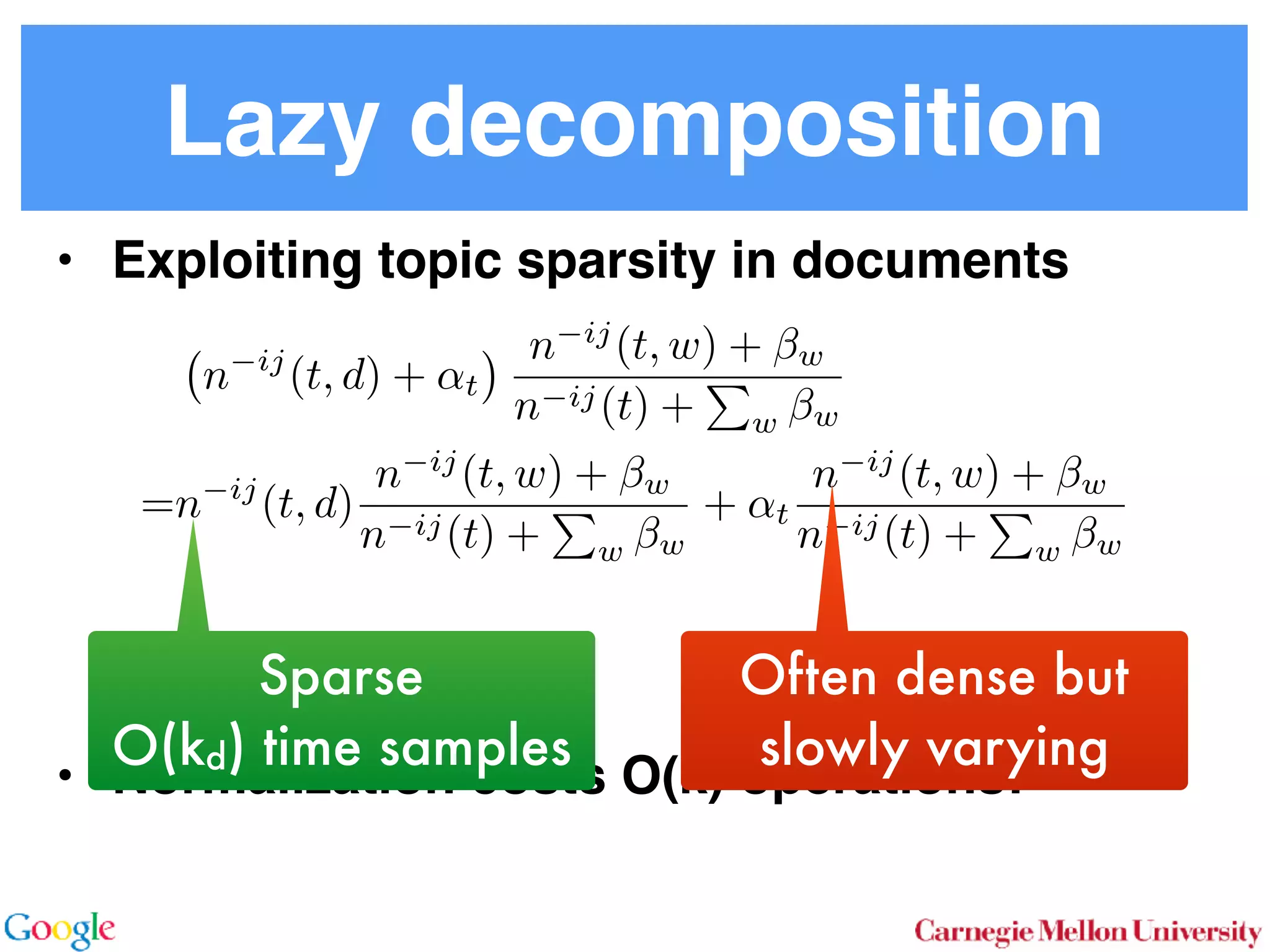
Lazy decomposition
• Exploiting topic sparsity in documents


• Normalization costs O(k) operations!
n ij
(t, d) + ↵t
n ij
(t, w) + w
n ij(t) +
P
w w
=n ij
(t, d)
n ij
(t, w) + w
n ij(t) +
P
w w
+ ↵t
n ij
(t, w) + w
n ij(t) +
P
w w
Sparse
O(kd) time samples
Often dense but
slowly varying
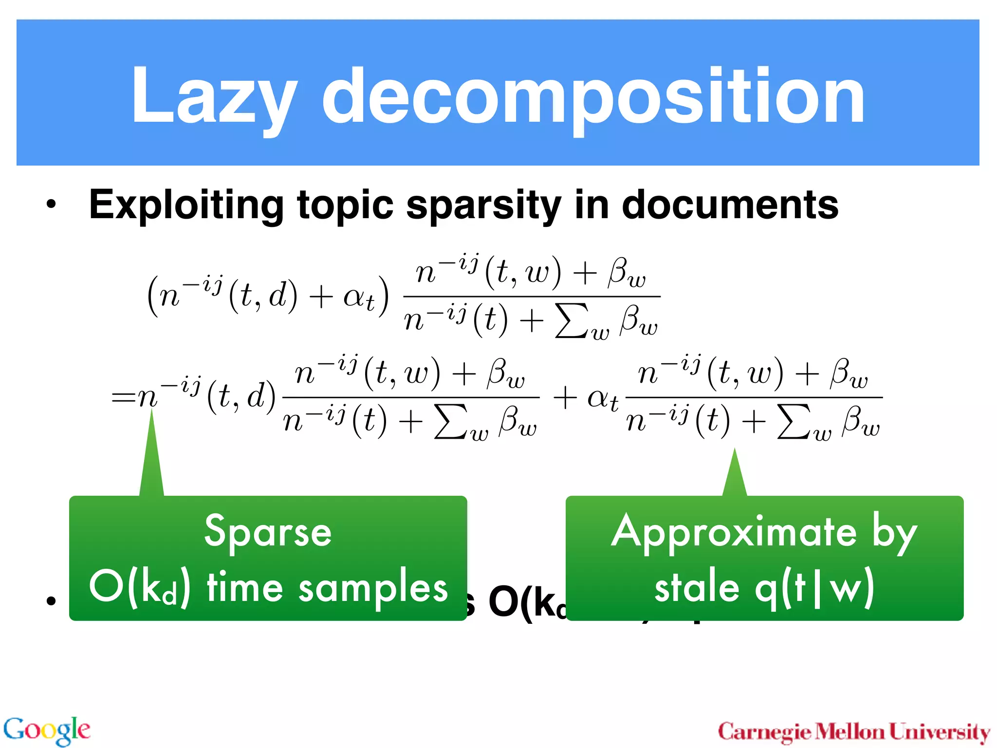
Lazy decomposition
• Exploiting topic sparsity in documents


• Normalization costs O(kd + 1) operations!
n ij
(t, d) + ↵t
n ij
(t, w) + w
n ij(t) +
P
w w
=n ij
(t, d)
n ij
(t, w) + w
n ij(t) +
P
w w
+ ↵t
n ij
(t, w) + w
n ij(t) +
P
w w
Sparse
O(kd) time samples
Approximate by
stale q(t|w)
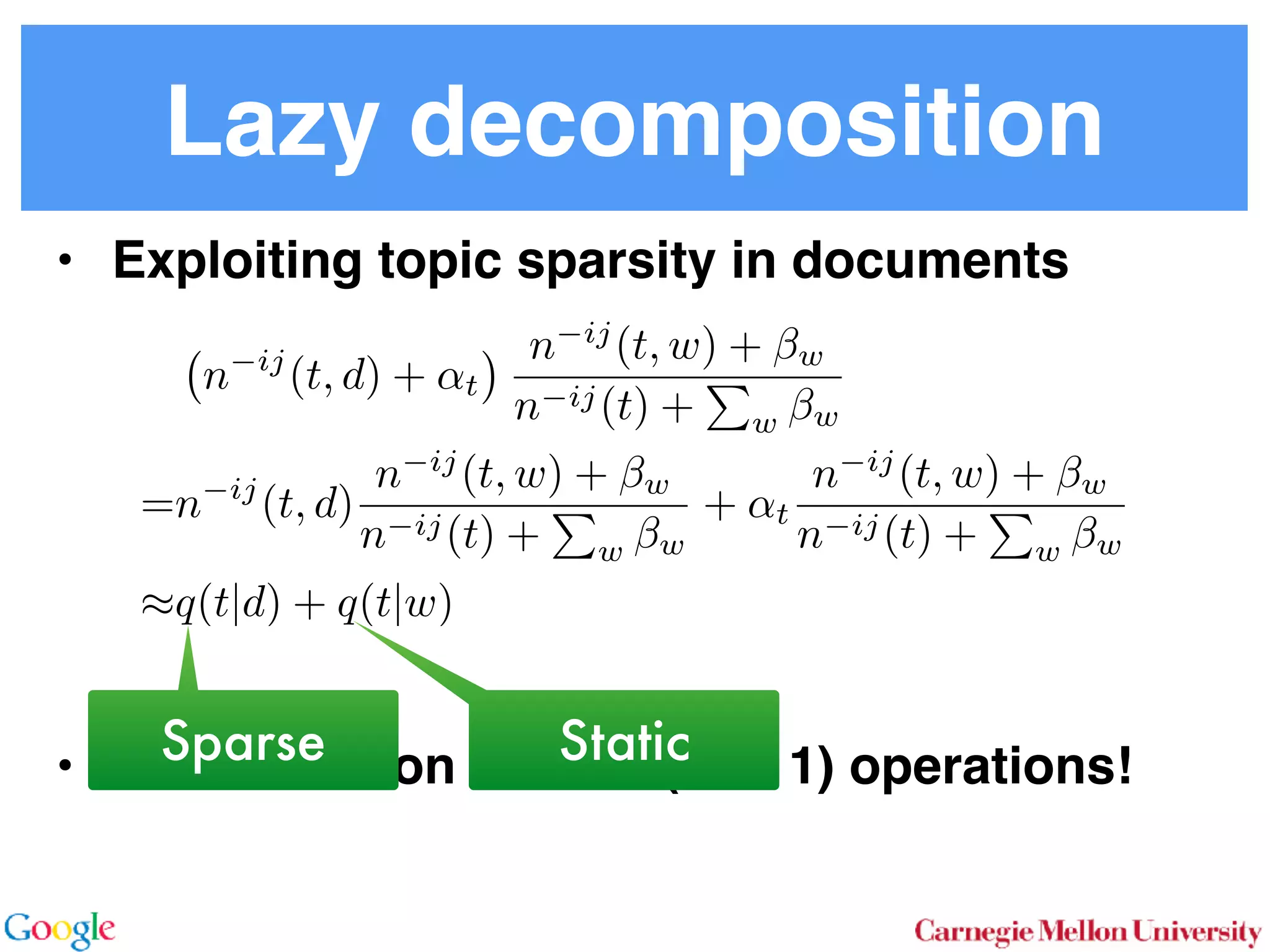
Lazy decomposition
• Exploiting topic sparsity in documents


• Normalization costs O(kd + 1) operations!Sparse
n ij
(t, d) + ↵t
n ij
(t, w) + w
n ij(t) +
P
w w
=n ij
(t, d)
n ij
(t, w) + w
n ij(t) +
P
w w
+ ↵t
n ij
(t, w) + w
n ij(t) +
P
w w
⇡q(t|d) + q(t|w)
Static
Metropolis Hastings

with stationary proposal distribution
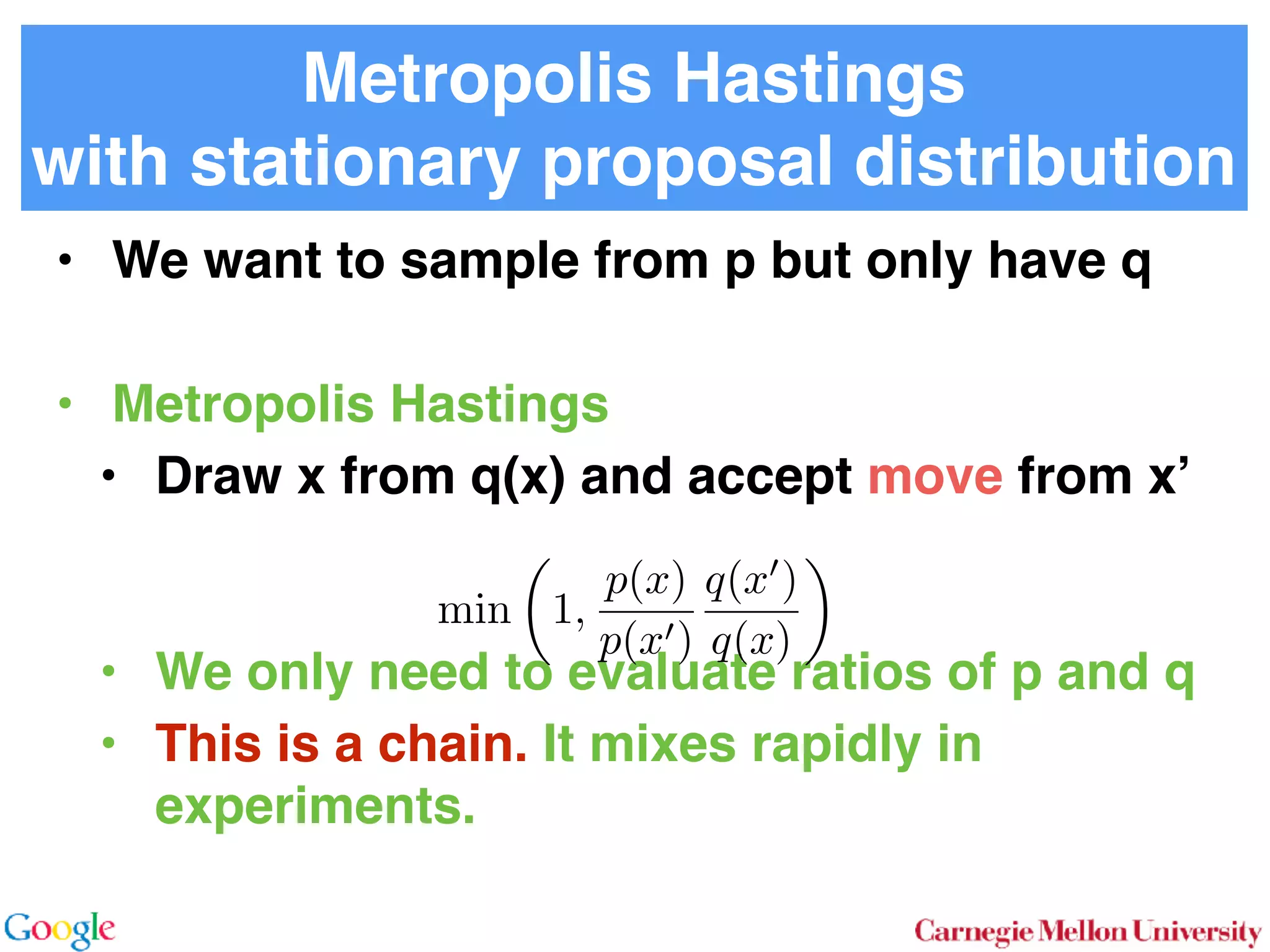
• We want to sample from p but only have q
• Metropolis Hastings
• Draw x from q(x) and accept move from x’


• We only need to evaluate ratios of p and q
• This is a chain. It mixes rapidly in
experiments.
min
✓
1,
p(x)
p(x0)
q(x0
)
q(x)
◆
Application to Topic Models
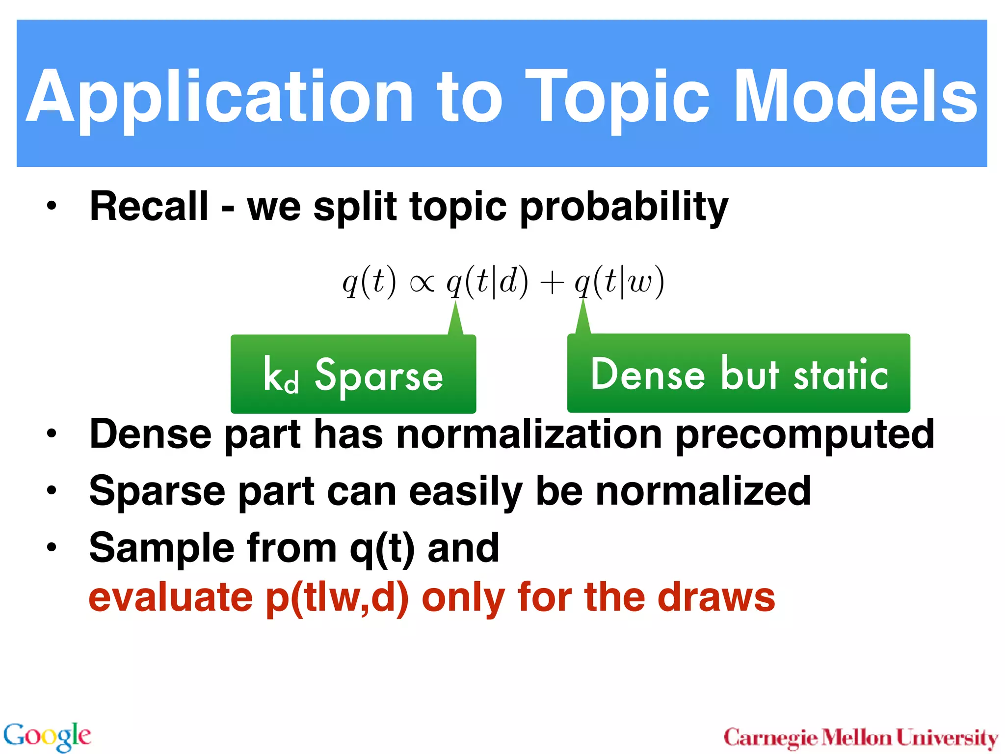
• Recall - we split topic probability
• Dense part has normalization precomputed
• Sparse part can easily be normalized
• Sample from q(t) and 

evaluate p(t|w,d) only for the draws
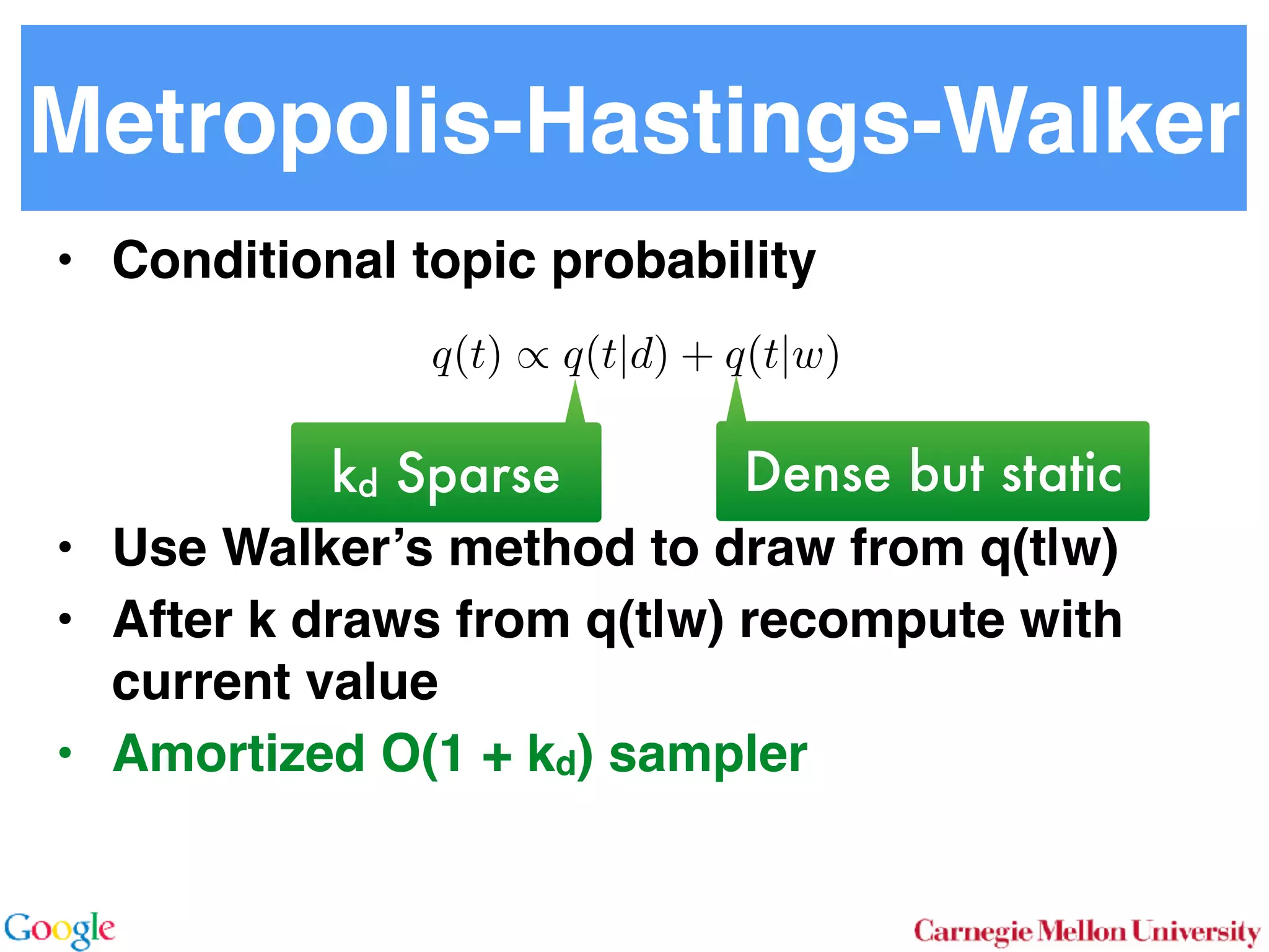
q(t) / q(t|d) + q(t|w)
kd Sparse Dense but static
In a nutshell
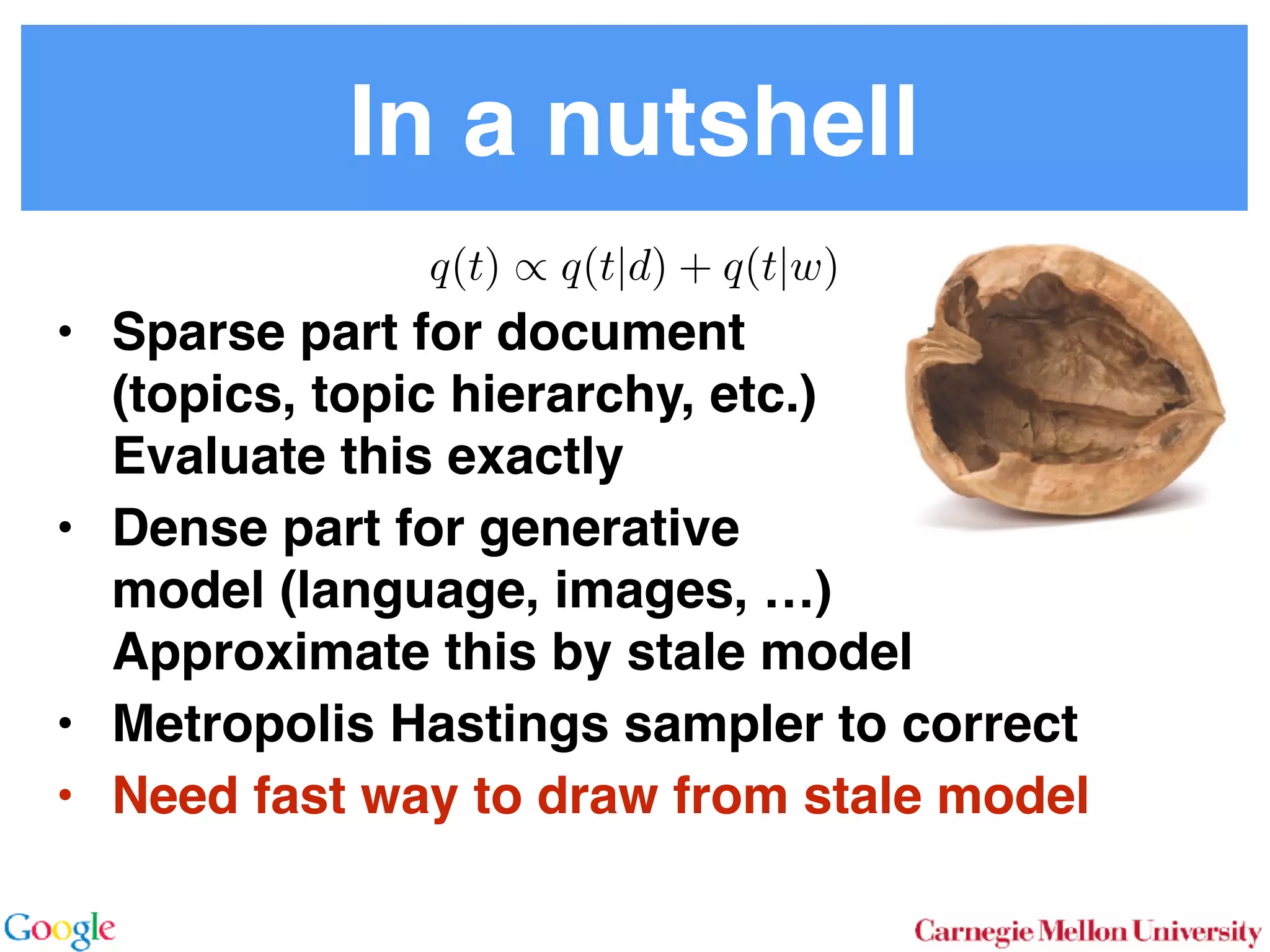
• Sparse part for document

(topics, topic hierarchy, etc.)

Evaluate this exactly
• Dense part for generative

model (language, images, …)

Approximate this by stale model
• Metropolis Hastings sampler to correct
• Need fast way to draw from stale model
q(t) / q(t|d) + q(t|w)
Sampling
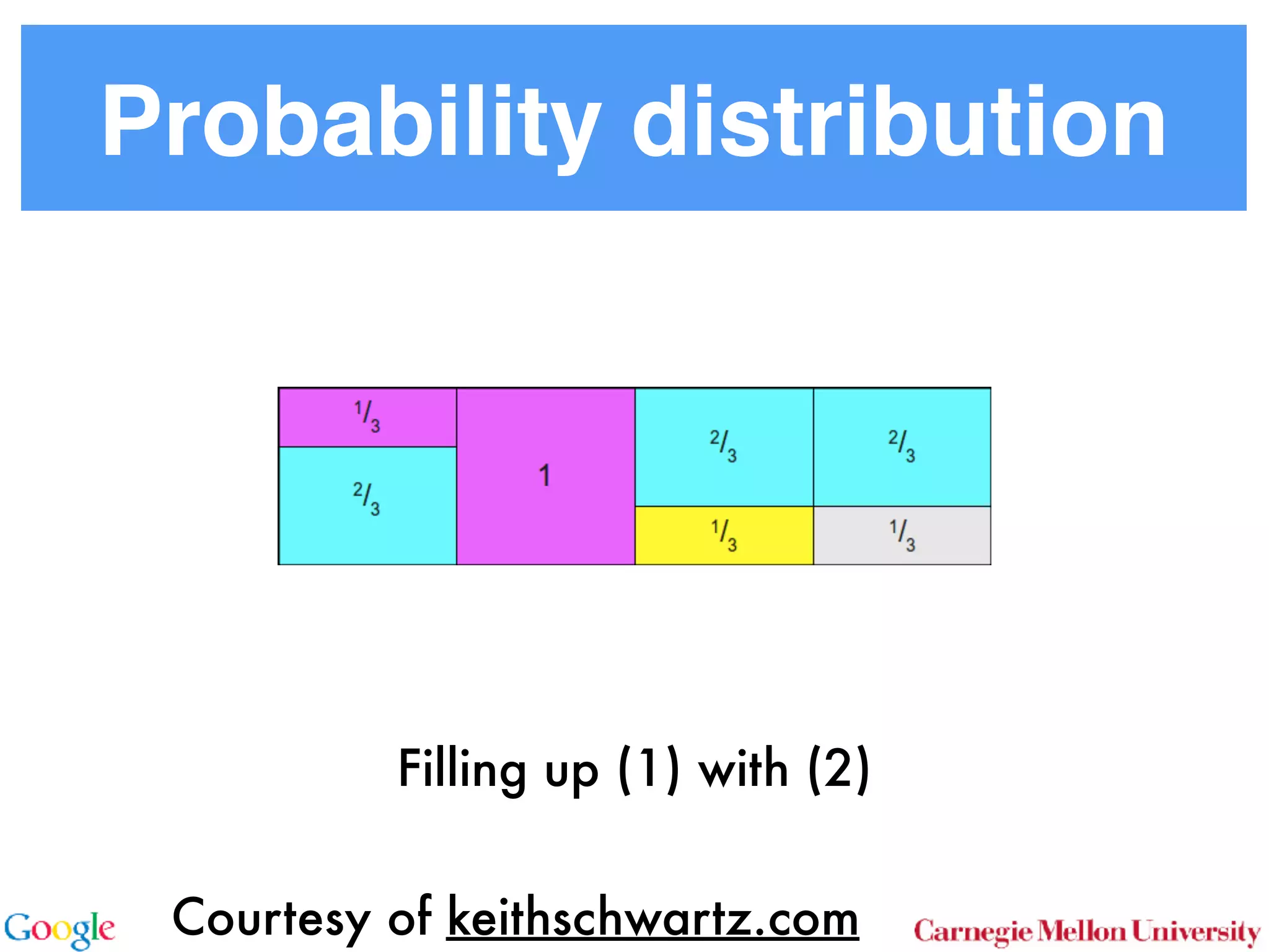
Walker’s Alias Method
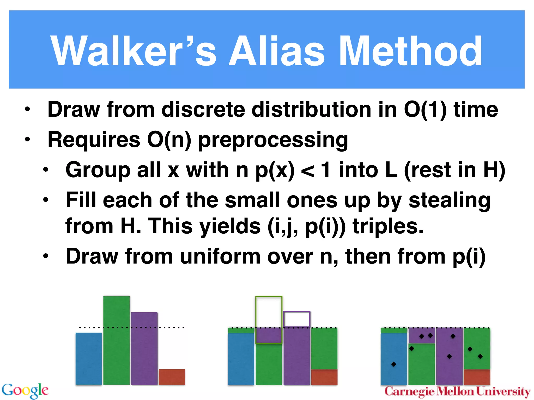
• Draw from discrete distribution in O(1) time
• Requires O(n) preprocessing
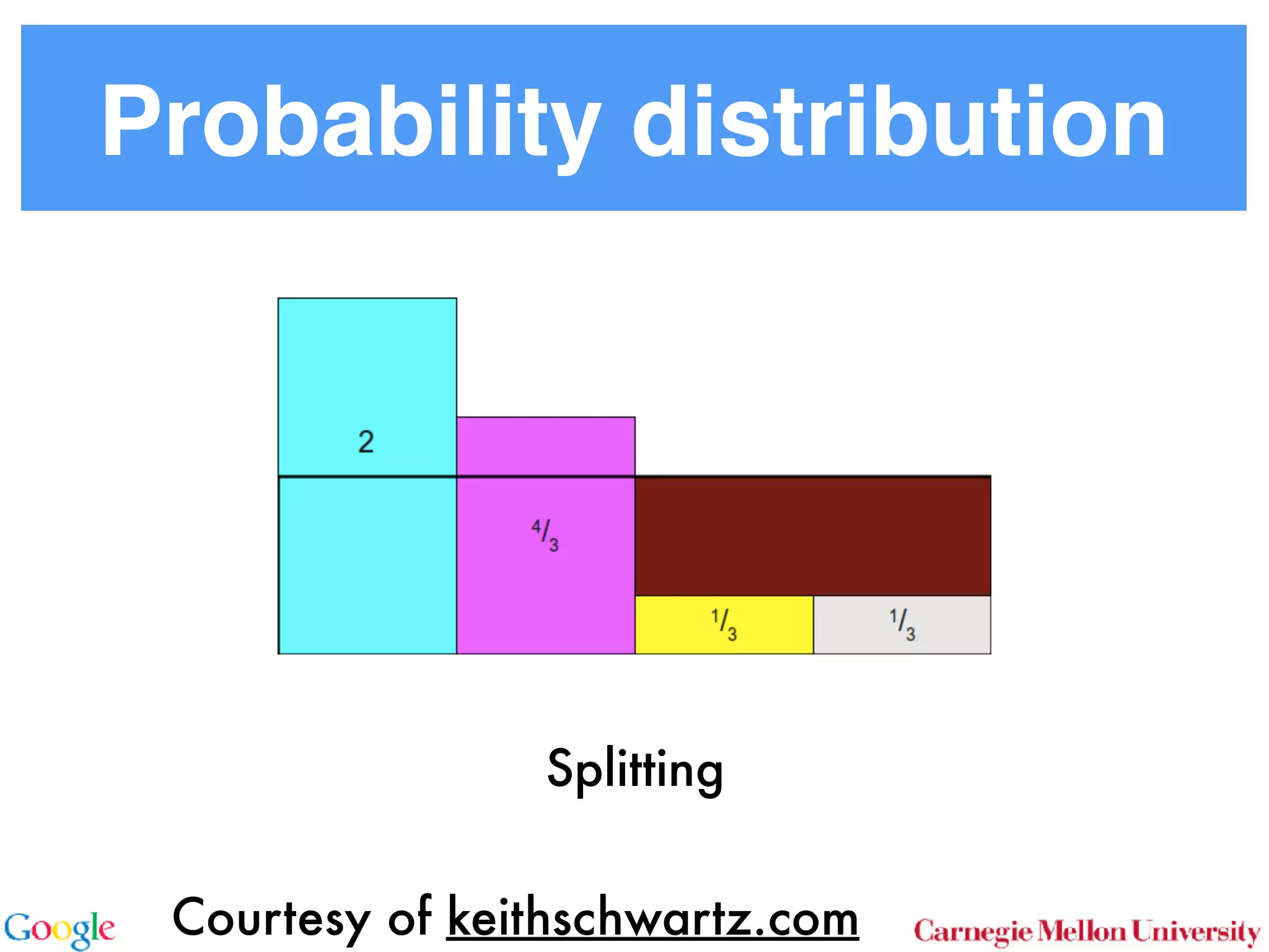
• Group all x with n p(x) < 1 into L (rest in H)
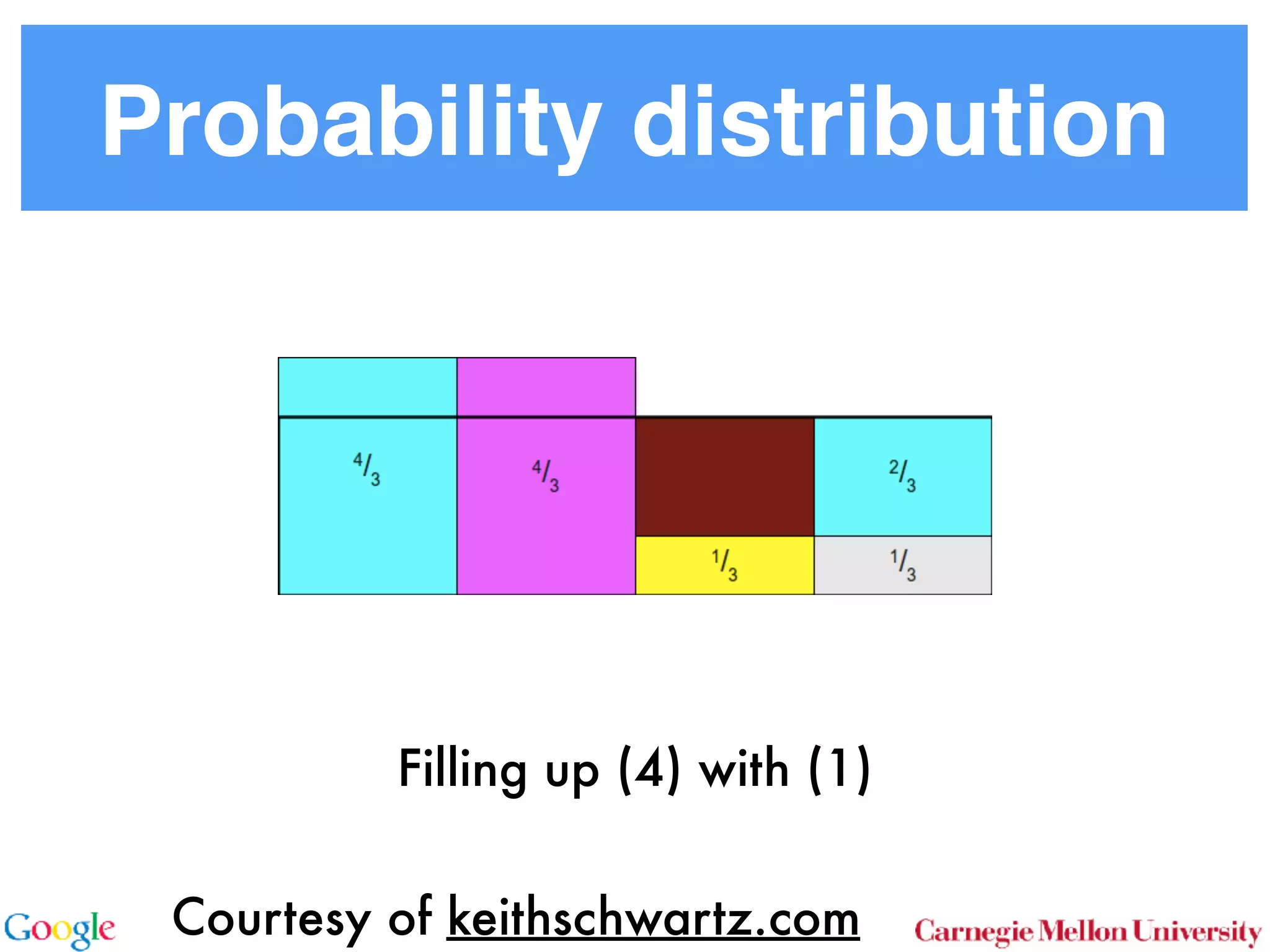
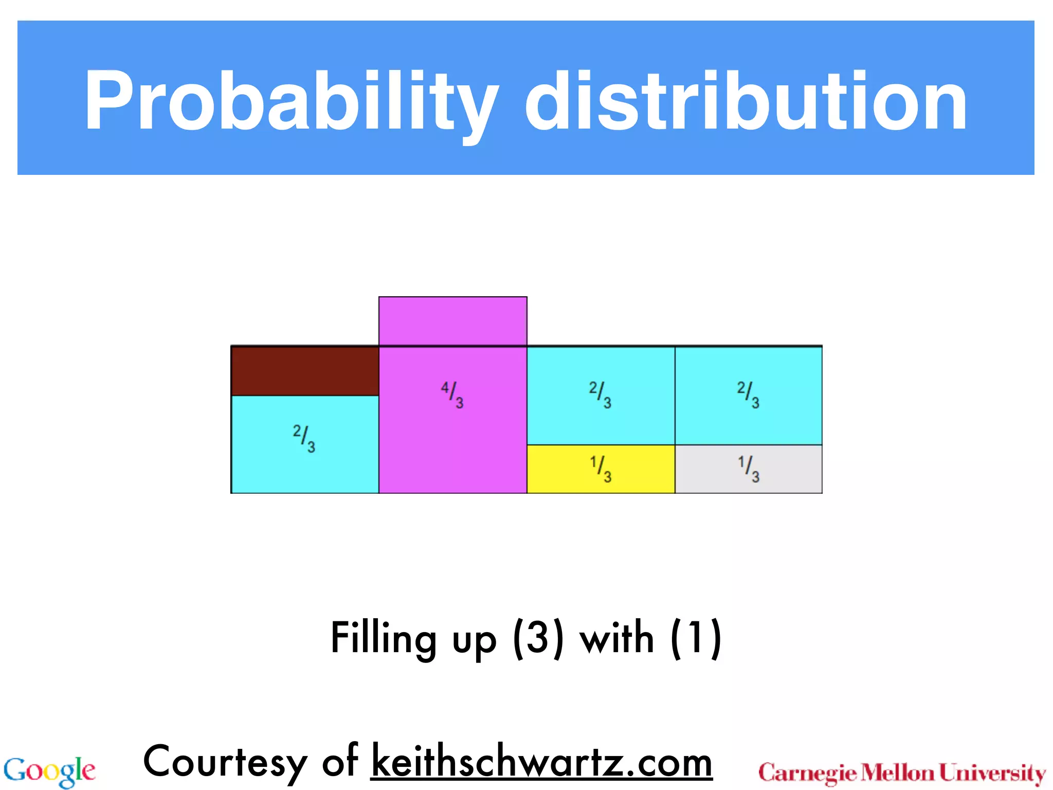
• Fill each of the small ones up by stealing
from H. This yields (i,j, p(i)) triples.
• Draw from uniform over n, then from p(i)
Probability distribution
Courtesy of keithschwartz.com
Probability distribution
Courtesy of keithschwartz.com
Splitting
Probability distribution
Courtesy of keithschwartz.com
Filling up (4) with (1)
Probability distribution
Courtesy of keithschwartz.com
Filling up (3) with (1)
Probability distribution
Courtesy of keithschwartz.com
Filling up (1) with (2)
Metropolis-Hastings-Walker
• Conditional topic probability
• Use Walker’s method to draw from q(t|w)
• After k draws from q(t|w) recompute with
current value
• Amortized O(1 + kd) sampler
q(t) / q(t|d) + q(t|w)
kd Sparse Dense but static
Experiments
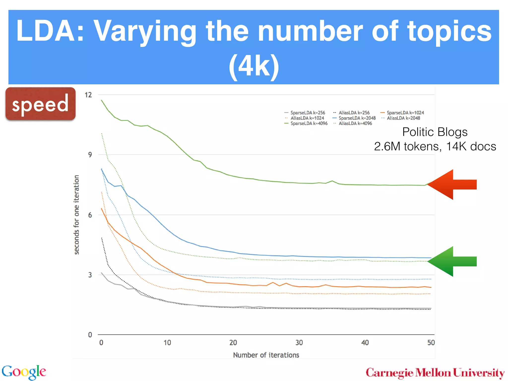
LDA: Varying the number of topics
(4k)
34%,
crease
tuition
ntw, th
the ali
than k
Politic Blogs
2.6M tokens, 14K docs
speed
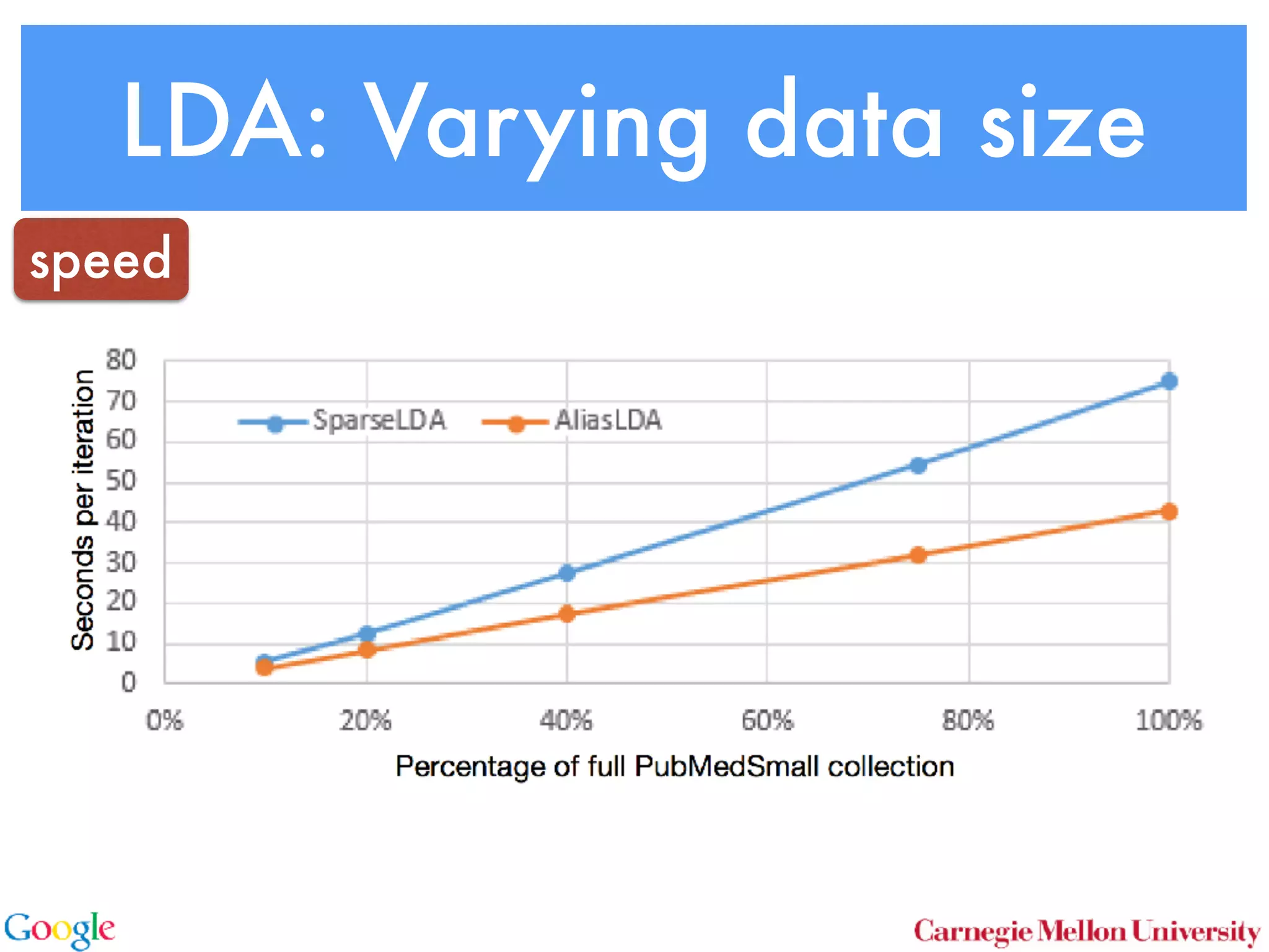
LDA: Varying data size
speed
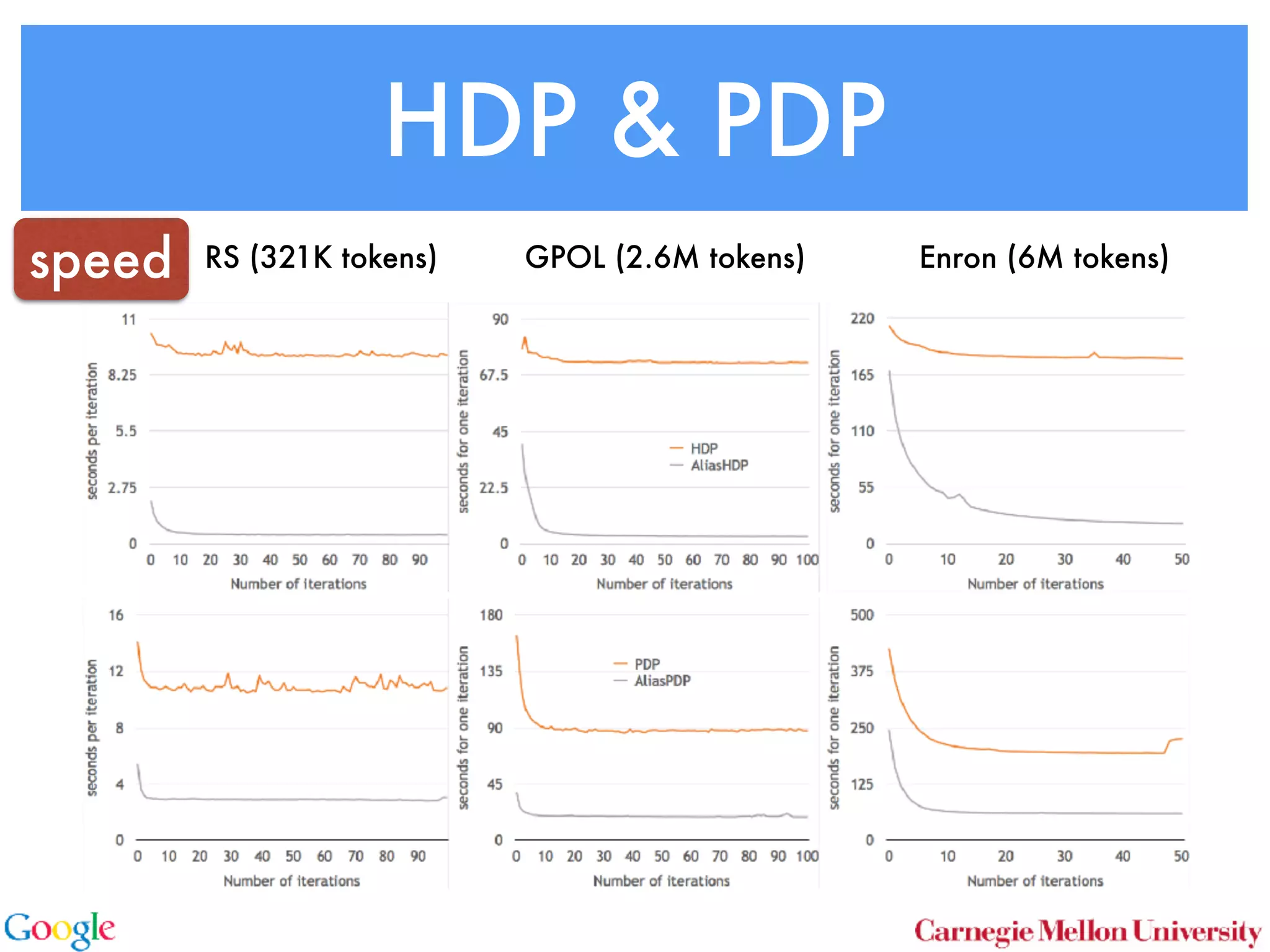
HDP & PDP
RS (321K tokens) GPOL (2.6M tokens) Enron (6M tokens)speed
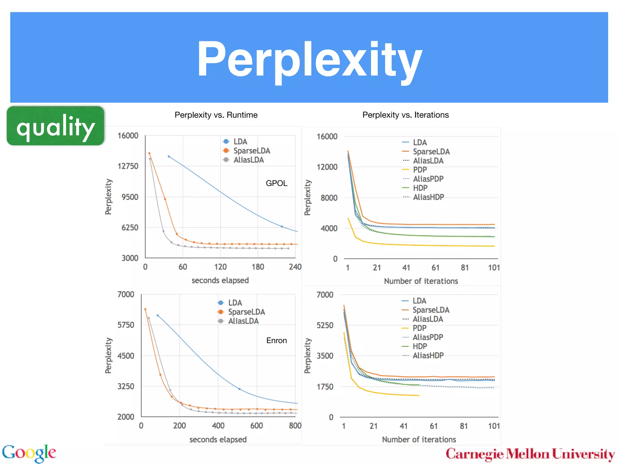
Perplexity
AliasLDA
opics for
34%, 37%, 41%, 43% respectively. In other words, it in-
creases with the amount of data, which conforms our in-
tuition that adding new documents increases the density of
ntw, thus slowing down the sparse sampler much more than
the alias sampler, since the latter only depends on kd rather
than kd + kw.
Perplexity vs. Runtime
GPOL
Enron
Perplexity vs. Iterations
quality
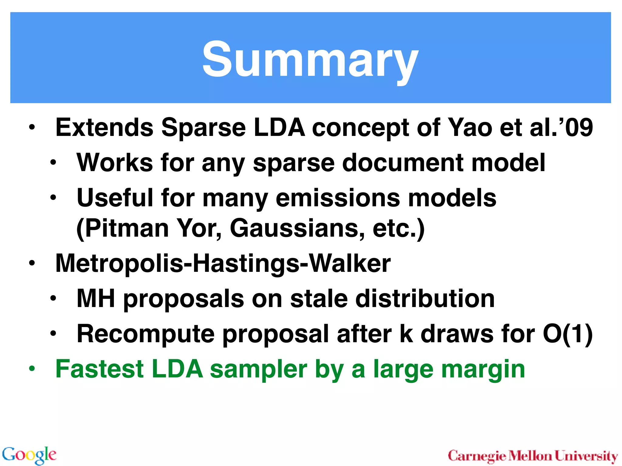
Summary
• Extends Sparse LDA concept of Yao et al.’09
• Works for any sparse document model
• Useful for many emissions models

(Pitman Yor, Gaussians, etc.)
• Metropolis-Hastings-Walker
• MH proposals on stale distribution
• Recompute proposal after k draws for O(1)
• Fastest LDA sampler by a large margin
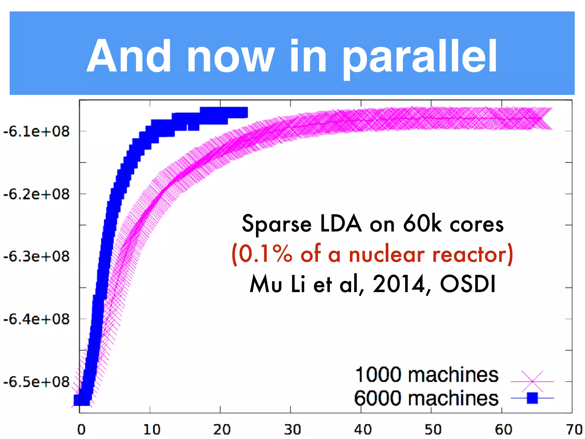
And now in parallel
Sparse LDA on 60k cores
(0.1% of a nuclear reactor)

Mu Li et al, 2014, OSDI
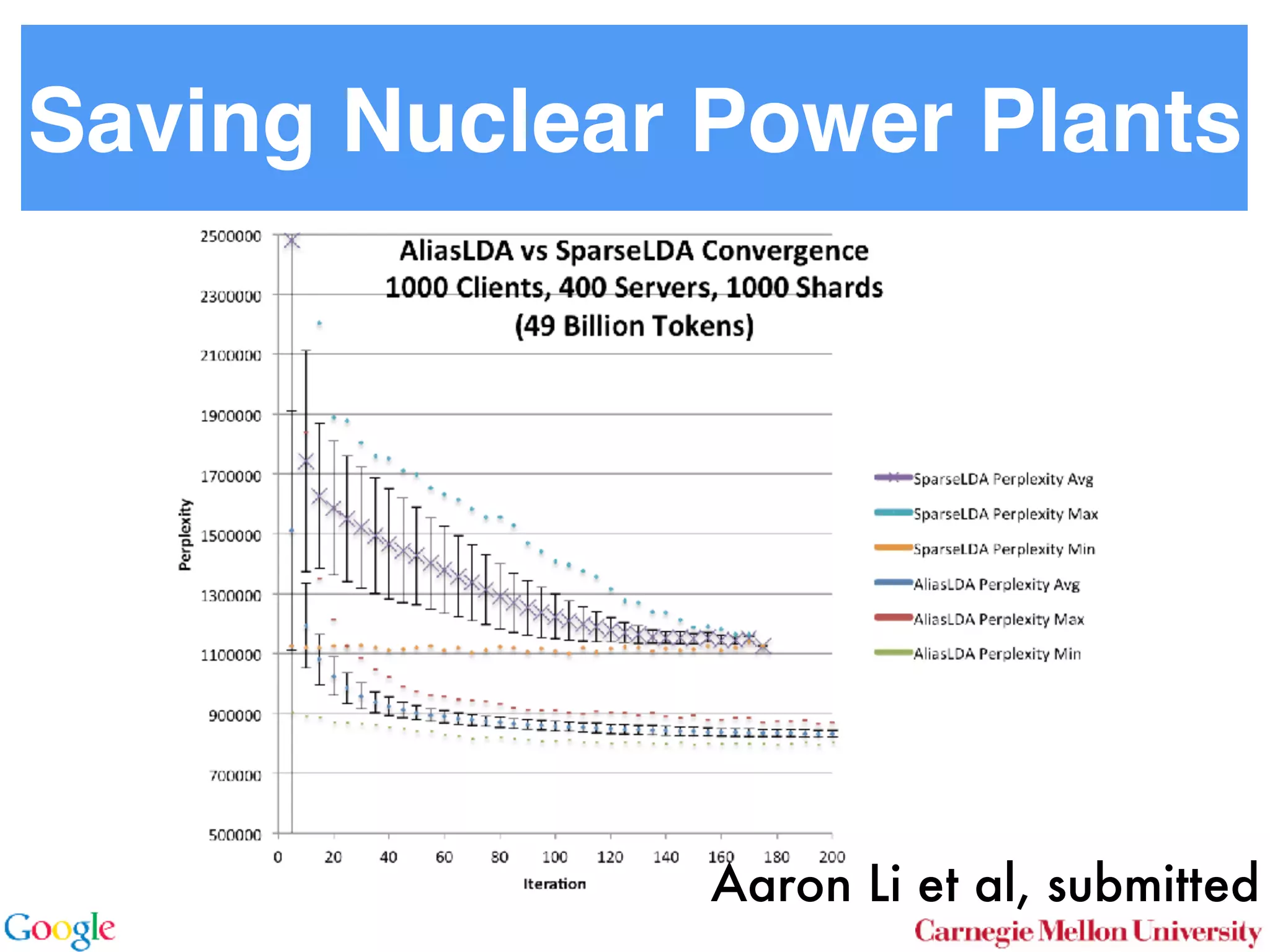
Saving Nuclear Power Plants
Aaron Li et al, submitted
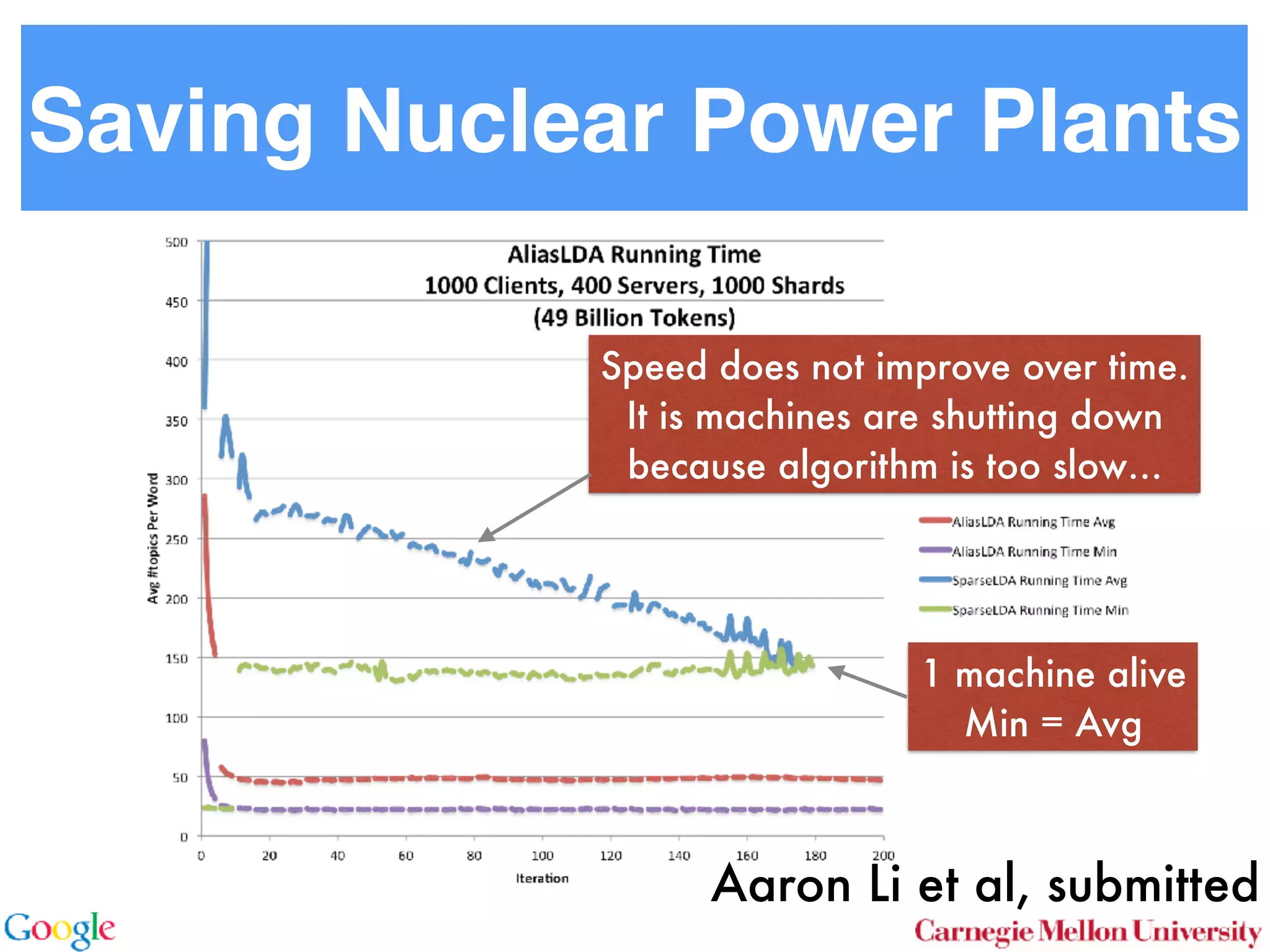
Saving Nuclear Power Plants
Aaron Li et al, submitted
Speed does not improve over time.
It is machines are shutting down
because algorithm is too slow…
1 machine alive
Min = Avg

KDD 2014 Presentation (Best Research Paper Award): Alias Topic Modelling (Reducing the Sampling Complexity of Topic Models)

  • 1.
    Reducing the Sampling Complexityof Topic Models Aaron Li joint work with Amr Ahmed, Sujith Ravi, Alex Smola CMU and Google
  • 2.
    Outline • Topic Models •Inference algorithms • Losing sparsity at scale • Inference algorithm • Metropolis Hastings proposal • Walker’s Alias method for O(kd) draws • Experiments • LDA, Pitman-Yor topic models, HPYM • Distributed inference
  • 3.
  • 4.
    Clustering & TopicModels Latent Dirichlet Allocation wij zij θi language prior topic probability topic label instance α β ψk
  • 5.
    Topics in text
 (Blei,Ng, Jordan, 2003)
  • 6.
    Collapsed Gibbs Sampler
 (Griffiths& Steyvers, 2005) wij zij θi language prior topic probability topic label instance α ψt β n ij (t, d) + ↵t n ij(d) + P t ↵t ⇥ n ij (t, w) + w n ij(t) + P w w
  • 7.
    • For eachdocument do • For each word in the document do • Resample topic for the word


 • Update (document, topic) table • Update (word,topic) table Collapsed Gibbs Sampler sparse for small collections sparse for most documents dense n ij (t, d) + ↵t ⇥ n ij (t, w) + w n ij(t) + ¯
  • 8.
    • For eachdocument do • For each word in the document do • Resample topic for the word


 • Update (document, topic) table • Update (word,topic) table Exploiting Sparsity
 (Yao, Mimno, Mccallum, 2009) sparse for small collections“constant” ↵t w n ij(t) + ¯ + n ij (t, d) n ij (t, w) + w n ij(t) + ¯ + n ij (t, w) ↵t n ij(t) + ¯ sparse for most documents amortized
 O(kd + kw) time
  • 9.
    • For eachdocument do • For each word in the document do • Resample topic for the word


 • Update (document, topic) table • Update (word,topic) table Exploiting Sparsity
 (Yao, Mimno, Mccallum, 2009) “constant” ↵t w n ij(t) + ¯ + n ij (t, d) n ij (t, w) + w n ij(t) + ¯ + n ij (t, w) ↵t n ij(t) + ¯ sparse for most documents dense for large collections O(k) time we solve this problem
  • 10.
    More Models • LDA •Poisson-Dirichlet Process 2.1 Latent Dirichlet Allocation In LDA [3] one assumes that documents are mixture dis- tributions of language models associated with individual topics. That is, the documents are generated following the graphical model below: for all i for all d for all k ↵ ✓d zdi wdi k For each document d draw a topic distribution ✓d from a Dirichlet distribution with concentration parameter ↵ ✓d ⇠ Dir(↵). (1) For each topic t draw a word distribution from a Dirichlet distribution with concentration parameter t ⇠ Dir( ). (2) For each word i 2 {1 . . . nd} in document d draw a topic from the multinomial ✓d via Sto sampl using ⌘tw a Unfor carefu dense Inst amort Here in O( numb tional does n gle wo chang the ba 2.2 To with m for all i for all d for all k ↵ ✓d zdi wdi t 0 In a conventional topic model the language model is sim- ply given by a multinomial draw from a Dirichlet distribu- tion. This fails to exploit distribution information between topics, such as the fact that all topics have the same common underlying language. A means for addressing this problem if n Her for rameter a prevents a word to be sampled too often by im- posing a penalty on its probability based on its frequency. The combined model described explicityly in [5]: ✓d ⇠ Dir(↵) 0 ⇠ Dir( ) zdi ⇠ Discrete(✓d) t ⇠ PDP(b, a, 0) wdi ⇠ Discrete ( zdi ) As can be seen, the document-specific part is identical to LDA whereas the language model is rather more sophisti- cated. Likewise, the collapsed inference scheme is analogous to a Chinese Restaurant Process [6, 5]. The technical di - culty arises from the fact that we are dealing with distribu- tions over countable domains. Hence, we need to keep track of multiplicities, i.e. whether any given token is drawn from i or 0. This will require the introduction of additional count variables in the collapsed inference algorithm. Each topic is equivalent to a restaurant. Each token in the document is equivalent to a customer. Each type of word corresponds each type of dish served by the restaurant. The same results in [6] can be used to derive the conditional probability by introducing axillary variables: • stw denotes the number of tables serving dish w in restaurant t. Here t is the equivalent of a topic. • rdi indicates whether wdi opens a new table in the restaurant or not (to deal with multiplicities). • mtw denotes the number of times dish w has been served in restaurant t (analogously to nwk in LDA). The conditional probability is given by: p(zdi = t, rdi = 0|rest) / ↵t + ndt bt + mt mtw + 1 stw mtw + 1 Smtw+1 stw,at Smtw stw,at (7) over topics. In other words, we add an extra level o chy on the document side (compared to the extra h on the language model used in the PDP). for all i for all d for al H ✓0 ✓d zdi wdi k More formally, the joint distribution is as follows: ✓0 ⇠ DP(b0, H(·)) t ⇠ Dir( ) ✓d ⇠ DP(b1, ✓0) zdi ⇠ Discrete(✓d) wdi ⇠ Discrete ( zdi ) By construction, DP(b0, H(·)) is a Dirichlet Process lent to a Poisson Dirichlet Process PDP(b0, a, H(·)) discount parameter a set to 0. The base distributio often assumed to be a uniform distribution in most At first, a base ✓0 is drawn from DP(b0, H(·)). T erns how many topics there are in general, and wh overall prevalence is. The latter is then used in the n of the hierarchy to draw a document-specific distrib that serves the same role as in LDA. The main di↵ that unlike in LDA, we use ✓0 to infer which topics popular than others. It is also possible to extend the model to more t levels of hierarchy, such as the infinite mixture mo Similar to Poisson Dirichlet Process, an equivalent Restaurant Franchise analogy [6, 19] exists for H cal Dirichlet Process with multiple levels. In this each Dirichlet Process is mapped to a single Chinese for all i for all d for all k d zdi wdi t 0 entional topic model the language model is sim- y a multinomial draw from a Dirichlet distribu- if no additional ’table’ is opened by word wdi. Otherwise p(zdi = t, rdi = 1|rest) (8 /(↵t + ndt) bt + atst bt + mt stw + 1 mtw + 1 + stw ¯ + st Smtw+1 stw+1,at Smtw stw,at Here SN M,a is the generalized Stirling number. It is given b
  • 11.
    More Models • LDA •Hierarchical-Dirichlet Process


 … even more mess for topic distribution 2.1 Latent Dirichlet Allocation In LDA [3] one assumes that documents are mixture dis- tributions of language models associated with individual topics. That is, the documents are generated following the graphical model below: for all i for all d for all k ↵ ✓d zdi wdi k For each document d draw a topic distribution ✓d from a Dirichlet distribution with concentration parameter ↵ ✓d ⇠ Dir(↵). (1) For each topic t draw a word distribution from a Dirichlet distribution with concentration parameter t ⇠ Dir( ). (2) For each word i 2 {1 . . . nd} in document d draw a topic from the multinomial ✓d via Sto sampl using ⌘tw a Unfor carefu dense Inst amort Here in O( numb tional does n gle wo chang the ba 2.2 To with m pus, the portional w from a ility dis- mon un- distribu- del, each base dis- anguage arameter le being ount pa- n by im- equency. 0) ntical to sophisti- nalogous cal di - distribu- ep track twice as large space of state variables. 2.3 Hierarchical Dirichlet Process To illustrate the e cacy and generality of our approach we discuss a third case where the document model itself is more sophisticated than a simple collapsed Dirichlet-multinomial. We demonstrate that there, too, inference can be performed e ciently. Consider the two-level topic model based on the Hierarchical Dirichlet Process [19] (HDP-LDA). In it, the topic distribution for each document ✓d is drawn from a Dirichlet process DP(b1, ✓0). In turn, ✓0 is drawn from a Dirichlet process DP(b0, H(·)) governing the distribution over topics. In other words, we add an extra level of hierar- chy on the document side (compared to the extra hierarchy on the language model used in the PDP). for all i for all d for all k H ✓0 ✓d zdi wdi k More formally, the joint distribution is as follows: ✓0 ⇠ DP(b0, H(·)) t ⇠ Dir( ) ✓d ⇠ DP(b1, ✓0) zdi ⇠ Discrete(✓d)
  • 12.
    Key Idea ofthe Paper • LDA
 
 
 • Approximate slowly changing distribution by fixed distribution. Use Metropolis Hastings • Amortized O(1) time proposals 2.1 Latent Dirichlet Allocation In LDA [3] one assumes that documents are mixture dis- tributions of language models associated with individual topics. That is, the documents are generated following the graphical model below: for all i for all d for all k ↵ ✓d zdi wdi k For each document d draw a topic distribution ✓d from a Dirichlet distribution with concentration parameter ↵ ✓d ⇠ Dir(↵). (1) For each topic t draw a word distribution from a Dirichlet distribution with concentration parameter t ⇠ Dir( ). (2) For each word i 2 {1 . . . nd} in document d draw a topic from the multinomial ✓d via Sto sampl using ⌘tw a Unfor carefu dense Inst amort Here in O( numb tional does n gle wo chang the ba 2.2 To with m slow changesbig variation
  • 13.
  • 14.
    Lazy decomposition • Exploitingtopic sparsity in documents


 • Normalization costs O(k) operations! n ij (t, d) + ↵t n ij (t, w) + w n ij(t) + P w w =n ij (t, d) n ij (t, w) + w n ij(t) + P w w + ↵t n ij (t, w) + w n ij(t) + P w w Sparse O(kd) time samples Often dense but slowly varying
  • 15.
    Lazy decomposition • Exploitingtopic sparsity in documents


 • Normalization costs O(kd + 1) operations! n ij (t, d) + ↵t n ij (t, w) + w n ij(t) + P w w =n ij (t, d) n ij (t, w) + w n ij(t) + P w w + ↵t n ij (t, w) + w n ij(t) + P w w Sparse O(kd) time samples Approximate by stale q(t|w)
  • 16.
    Lazy decomposition • Exploitingtopic sparsity in documents


 • Normalization costs O(kd + 1) operations!Sparse n ij (t, d) + ↵t n ij (t, w) + w n ij(t) + P w w =n ij (t, d) n ij (t, w) + w n ij(t) + P w w + ↵t n ij (t, w) + w n ij(t) + P w w ⇡q(t|d) + q(t|w) Static
  • 17.
    Metropolis Hastings
 with stationaryproposal distribution • We want to sample from p but only have q • Metropolis Hastings • Draw x from q(x) and accept move from x’
 
 • We only need to evaluate ratios of p and q • This is a chain. It mixes rapidly in experiments. min ✓ 1, p(x) p(x0) q(x0 ) q(x) ◆
  • 18.
    Application to TopicModels • Recall - we split topic probability • Dense part has normalization precomputed • Sparse part can easily be normalized • Sample from q(t) and 
 evaluate p(t|w,d) only for the draws q(t) / q(t|d) + q(t|w) kd Sparse Dense but static
  • 19.
    In a nutshell •Sparse part for document
 (topics, topic hierarchy, etc.)
 Evaluate this exactly • Dense part for generative
 model (language, images, …)
 Approximate this by stale model • Metropolis Hastings sampler to correct • Need fast way to draw from stale model q(t) / q(t|d) + q(t|w)
  • 20.
  • 21.
    Walker’s Alias Method •Draw from discrete distribution in O(1) time • Requires O(n) preprocessing • Group all x with n p(x) < 1 into L (rest in H) • Fill each of the small ones up by stealing from H. This yields (i,j, p(i)) triples. • Draw from uniform over n, then from p(i)
  • 22.
  • 23.
    Probability distribution Courtesy ofkeithschwartz.com Splitting
  • 24.
    Probability distribution Courtesy ofkeithschwartz.com Filling up (4) with (1)
  • 25.
    Probability distribution Courtesy ofkeithschwartz.com Filling up (3) with (1)
  • 26.
    Probability distribution Courtesy ofkeithschwartz.com Filling up (1) with (2)
  • 27.
    Metropolis-Hastings-Walker • Conditional topicprobability • Use Walker’s method to draw from q(t|w) • After k draws from q(t|w) recompute with current value • Amortized O(1 + kd) sampler q(t) / q(t|d) + q(t|w) kd Sparse Dense but static
  • 28.
  • 29.
    LDA: Varying thenumber of topics (4k) 34%, crease tuition ntw, th the ali than k Politic Blogs 2.6M tokens, 14K docs speed
  • 30.
  • 31.
    HDP & PDP RS(321K tokens) GPOL (2.6M tokens) Enron (6M tokens)speed
  • 32.
    Perplexity AliasLDA opics for 34%, 37%,41%, 43% respectively. In other words, it in- creases with the amount of data, which conforms our in- tuition that adding new documents increases the density of ntw, thus slowing down the sparse sampler much more than the alias sampler, since the latter only depends on kd rather than kd + kw. Perplexity vs. Runtime GPOL Enron Perplexity vs. Iterations quality
  • 33.
    Summary • Extends SparseLDA concept of Yao et al.’09 • Works for any sparse document model • Useful for many emissions models
 (Pitman Yor, Gaussians, etc.) • Metropolis-Hastings-Walker • MH proposals on stale distribution • Recompute proposal after k draws for O(1) • Fastest LDA sampler by a large margin
  • 34.
    And now inparallel Sparse LDA on 60k cores (0.1% of a nuclear reactor)
 Mu Li et al, 2014, OSDI
  • 35.
    Saving Nuclear PowerPlants Aaron Li et al, submitted
  • 36.
    Saving Nuclear PowerPlants Aaron Li et al, submitted Speed does not improve over time. It is machines are shutting down because algorithm is too slow… 1 machine alive Min = Avg