Land suitability

1. Land Suitability Analysis
Lecturer: Ms Judy Kawira

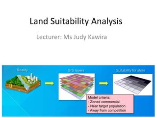
2. Introduction
• The Land Suitability Analysis (LSA) project is a GIS-based
process for evaluating the suitability of land for
development.
• The two major outputs of the LSA project are an
environmental composite map and a land suitability
map.
• The environmental composite map shows the extent and
overlap of natural features and environmental conditions
that indicate the capability and limitations of natural
systems for urban development.
• The land suitability map shows the relative suitability of
land in a planning area for urban-type development.

3. • Land suitability analysis is a mandatory component of
the local land use plan.
• It is a process for determining a planning area's supply
of land that is suitable for development.
• The analysis includes consideration of a number of
factors, including natural system constraints,
compatibility with existing land uses and development
patterns, existing land use policies, and the availability
of community facilities.
• A key output of the analysis is a land suitability map
that shows vacant or under-utilized land that is suited
for the development.
• This map is a major part of the foundation for the
development of local land use policies and the future
land use map.

4. GIS Approach
• Land suitability analysis involves the application of
criteria to the landscape to assess where land is
most and least suitable for development of
structures and infrastructure.
• The system enables planners to create and modify
a land suitability analysis that makes the best use
of available data.

5. GIS Tools for Land Suitability Analysis
i. GIS and Spatial Analysis
• In addition to storing, retrieving, displaying spatial
data, a geographic information system enables the
user to create buffers, overlays, intersections,
proximity analysis, spatial joins, map algebra, and
other analytical operations.
• In the context of land suitability, GIS helps the user
determine what locations are most/least suitable
for development.
• In this way, the results of GIS analysis can provide
support for decision-making.

6. • The eight steps in Spatial Analysis include:
a) Define criteria for the analysis
b) Define data needed
c) Determine what GIS analysis operations should
be performed
d) Prepare the data
e) Create a model
f) Run the model
g) Analyze results
h) Refine the model as needed

7. ii. Raster vs. Vector Approach
• There are two possible data models that can be used in a
GIS: vector and raster.
• The raster data model represents features as a matrix of
cells (pixels) in continuous space.
• Vector data consist of discrete points, lines, and polygons.
These feature shapes are defined by x and y coordinates.
• Raster data are used for land suitability modeling because
analysis can be performed on several raster layers at once.
• For example, raster data enable the user to perform a
weighted overlay on several layers. Vector data enable
analysis on only two layers at a time in an operation
thatrequires a great deal of computer resources.
• Raster data provide continuous coverage of a geographic
area and analysis is much more efficient.

8. Technical Issues with a Raster Data
Model
Resolution
• The cell size used for a raster layer will affect the results of the
analysis and how the map looks.
• The cell size should be based on the original map scale and
the minimum mapping unit.
• Using too large a cell size will cause some information to be
lost.
• Using a cell size that is too small requires a lot of storage
space, and takes longer to process, without adding additional
precision to the map.
• For a given analysis, you will need to decide the optimal
resolution to maximize accuracy and performance.
• The higher the resolution, the greater the accuracy; but
performance suffers.

9. Pixels contain one value only
• Limiting a cell to one value can misrepresent
spatial data.
• For example, the boundary of two soil types
may run across the middle of a cell.
• In such cases, the cell is given the value of the
largest fraction of the cell, or the value of the
middle point in the cell.

10. Only one item of information is available for each
location within a single layer
Multiple items of information require multiple
layers.
If, in a soils vector layer, you have two attributes—
septic suitability and flood frequency--you will
have to create two raster layers: one that contains
septic suitability information and one that contains
flood frequency information.

11. Discrete and continuous phenomena
• Discrete phenomena
Landuse
Ownership
Political boundaries
• Continuous phenomena
Elevation
Distance
Density
Suitability

12. iii. Introduction to Spatial Analyst
• The ESRI Spatial Analyst extension enables the user to
create, query, map, and analyze cell-based raster data and
to perform integrated vector–raster analysis.
• Spatial Analyst enables desktop GIS users to create, query,
and analyze cell-based raster maps; derive new
information from existing data; query information across
multiple data layers; fully integrate cell-based raster data
with traditional vector data sources; and create
sophisticated spatial models using ModelBuilder.
• For the Land Suitability Analysis, users can rate areas
according to several factors with varying weights and
values, and derive new information from existing data to
determine land suitability.

13. • Additional capabilities available through the standard
user interface include queries on multiple grid
themes, neighborhood and zone analysis, grid
classification and display, summary histograms, and
more.
• Operations available with Spatial Analyst:
 Convert feature themes (point, line, or polygon) to
grids
 Create raster buffers based on distance from any
raster or vector feature
 Create density maps of point features
 Perform Boolean queries and algebraic calculations
on multiple grid themes simultaneously
 Do neighborhood and zone analysis
 Display and reclassify grid data

14. iv. Introduction To Model Builder
ModelBuilder is a tool for creating and managing automated
and self-documenting spatial models.
Modelbuilder enables users to create process- flow diagrams
and scenarios to automate the modeling process.
Users can easily change the data sets used by the model,
modify the influence of each data set on the model, perform
complex analysis functions, and generate maps that illustrate
the results of analysis.
Data derived from one model can be used as input for another
model.
Users can run a model with a variety of parameters to assess
data sensitivity or to evaluate geographically different but
structurally similar data sets.
Users can copy portions of their models within a model and
smaller models can be combined to build larger models.

15. • In the case of Land Suitability Analysis, the layer
weights can be easily changed, and the models may
be re-run to evaluate the new results.
• ModelBuilder is ideal for this task because it allows
users to overlay multiple layers, rank order
categories within each layer, include a weight for
each layer, and sum using map algebra.
• ModelBuilder creates a process-flow diagram that
displays the layers and operations.
• For example, the land suitability model combines
and classifies multiple GIS layers to produce a land
suitability map as illustrated in the figure below.

16. Model Builder Example

17. Land
Suitability
Model

18. Define the Criteria
• criteria for the Land Suitability Analysis is
based on the Guidelines set and modified
criteria according to available datasets.
• The criteria for suitability for development
(high, medium, low, and least suitable) can be
identified as follows:
• Within 100-year Flood Zones have low
development suitability

19. • Within Water Supply Watersheds have low suitability
• Within 500 feet of a Significant Natural Heritage Area have low
suitability
• Within 500 feet of a Hazardous Substance Disposal Site have low
suitability
• Within 500 feet of a Wastewater Treatment Plant have low
suitability
• Within 500 feet of a Municipal Sewage Discharge Point have low
suitability
• Within 500 feet of a Land Application Site have low suitability
• Within 500 feet of an Airport have low suitability
• Within a half-mile of Primary Roads have high suitability; within
a half-mile to a mile have medium suitability; areas greater than
one mile outside of primary roads have low suitability
• Within a half-mile of Developed Land have high suitability; areas
within a half-mile to a mile have medium suitability; areas
further than one mile away from developed land have low
suitability

20. • Within a quarter-mile of Water Pipes have high
suitability; areas within a quarter-mile to a half-mile
of water pipes have medium suitability; areas further
than a half-mile away from water pipes have low
suitability
• Within a quarter-mile of Sewer Pipes have high
suitability; areas within a quarter-mile to a half-mile
of sewer pipes have medium suitability; areas further
that a half-mile away from water pipes have low
suitability
• Within government reserves or State Lands are
LEAST suitable
• Within Protected Lands are LEAST suitable
• Within Estuarine Waters are LEAST suitable

21. • According to these criteria, values for layers are quantitatively
scored according to suitability for development.
• For example, an area that is inside a storm surge area or within
500 feet of a Significant Natural Heritage Area has low
suitability. These areas receive a score of –2 (negative 2).
• An area that is close to existing infrastructure (roads, sewer
lines, existing development, etc.) has high suitability for
development. These areas receive a score of +2 (positive two).
• Note that the proximity concept is represented by a buffer in
the model. A buffer should not be smaller than the distance of
one side of a cell. In this case, the smallest buffer is 500 feet
and a cell has a width of 209 feet.
• Also, to account for proximity of features to cells on the
boundaries of the study area (county), themes that are subject
to buffers are clipped to a polygon of the county plus 2 miles (2-
mile buffer of county boundary including the county).
• The final map will be clipped to the county boundary (not
buffered).

22. • Additionally, most the data layers are ranked according to
how important they are to the overall analysis.
• In the criteria spreadsheet developed in the Table below,
users may rank a layer as 1, 2 or 3, with 3 being very
important.
• Other values may be used, but keep in mind the
advantage of keeping the factors relatively uncomplicated
for presentation and explanation in public meetings.
• The least suitable areas (protected lands, military areas,
coastal wetlands, estuarine waters, and exceptional and
substantial non-coastal wetlands) are treated somewhat
differently.
• They are given scores of 0 or 1. Areas within protected
lands, coastal wetlands, etc., receive a score of 0. Areas
outside of these sensitive areas receive a score of 1.

23. Criteria
Table
Example
Note that the first set of
layers (green shading) are
either least suitable (the
value of zero will be
multiplied by the results of
the layers with white and
gray shading for a product
of zero) or medium
suitability (the value of one
will be multiplied by the
results of the other sets of
layers for a product equal
to the score based on
those other sets).

24. • The next step is to rank the layers from 1 to 3 with 3 representing the
most weight in land suitability.
• The spreadsheet included on the Land Suitability CD is ready for the user
to modify the default weights (see the next Table).
• Once a ranking is agreed upon, the model requires that the user
quantify the ranked layers from an ordinal scale (ranked 1 thru 3) to a
percentage of the total (percent weight) to assign relative weights.
• The relative weight for a layer is equal to 100 (percent) divided by the
product of the sum of all rankings times the ranking for that layer.
• In other words, it is the whole pie divided by the number of pieces
(yielding the size of a piece), times the number of pieces for that layer.
• If all layers were assigned a weight of 1, the relative weight in percent
for any one layer would be equal to the 100 divided by the number of
layers (one equal piece of pie each).
• The far right column of the spreadsheet expresses the relative weights
as a ratio (or “multiplier” required for the model, below).
• Note that these numbers change for each county depending on the
number of layers that apply. The calculations are already set in formulas
in the spreadsheet.

25. Example of
Rankings
and Percent
Weights

26. Define the Data
• The final determination of the factors
included in the analysis is influenced by the
availability of digital data layers.
• The data are projected to one datum in order
to have similar coordinate system

27. Determine the GIS Operations
• Based on the established criteria and data, the next
step is to define what operations need to be
performed in order to determine land suitability.
• Many layers will have to be converted from vector
to raster.
• Once in raster format, each layer’s values need to
be reclassified into either the 1’s and 0’s scoring
system, or the –2 thru +2 scoring system.
• Buffering will have to be done on many layers to
determine what values should be assigned
inside/outside the extent of the feature and it’s
buffer.
• For example, airports are buffered by 500 feet.
Any areas within that buffer are assigned a value of
–2; areas outside are assigned a value of +2.

28. Operations used in this analysis:
• Raster to Vector Conversion
• Buffer
• Reclassification
• Map Algebra – multiply by a constant (absolute
weight)
• Map Algebra – add multiple layers
• Map Algebra – multiply layers

29. • Vector to Raster Conversion:
• Layers must be converted from vector to raster to
be used in the model.
• Some layers are converted within the model itself.
Others have already been converted outside of
the model.

30. • Buffer:
• Many criteria specify that areas within a
specific feature have suitability; outside have
high suitability (and vice-versa).
• Example: Areas within 500 feet of a Hazardous
Substance Disposal Site have low suitability.
Example: Areas within 500 feet of a Hazardous Substance Disposal Site have low
suitability.

31. • Reclassify:
• Some layers need to be reclassified. For example,
the ‘Soils With Septic Limitations’ layer has a
‘septic’ attribute that contains values, Severe,
Moderate, or Slight.
• These values are reclassified to –2, 1, and +2
respectively.

32. • Map Algebra
• Multiply by a constant: The weighted layers will
each be multiplied by their respective absolute
weight. For example, all the values in the Storm
Surge Areas will be multiplied by 0.08696
assuming the criteria listed above

33. • Map Algebra – Add Multiple Layers:
• After all weighted layers are multiplied by their
respective constants, they will be added together
to get a suitability rating. The following example
shows only two of the layers being added (allow
for rounding in addition). When all layers are
added, the resultant layer has values from – 2 to
+2.

34. • Map Algebra – Multiply Layers: Layers that have
features to be scored least suitable are classified
with 0’s and 1’s, then the layers multiplied
together. The resulting layer shows all areas least
suitable for development.
Multiply the reclassified county
boundary with the land
suitability. The No Data values
will drop out, clipping the land
suitability map.

35. Data Preparation
• After the GIS operations are determined, the
data must be prepared for the Model.
• This includes clipping the data to the correct
boundary; creating subsets of data such as
coastal wetlands versus all wetlands; and even
converting some data to raster format before it
is added to the model.

36. Using ModelBuilder
• Map document files (.mxd) are provided for
the ArcGIS models. The model is located in a
new Toolbox in ArcToolbox (LSA Model and
Environmental Composite Model). To run or
make edits to the model – double click the
Toolbox function and right click the model and
select Edit. A new window will open. This is
the Model Builder interface.

37. Running the Land Suitability Model

38. Evaluating the Results
• ArcMap permits the classification of results by natural
breaks, equal intervals, etc.
• Natural breaks is a better classification of the results.
• Natural breaks are best for comparing relative suitability of
resources within specific planning area within a county
• Equal intervals may mask subtle differences between
suitability of locations within the planning area
• Equal interval may mean that some areas have few or no
areas suitable for development
• Significant research may be required to determine ranges
or the ranges would be more arbitrary than natural breaks
• Natural breaks appear to be more statistically valid than
equal intervals

39. • Verify the results by viewing the newly classified
grid underneath the vector layers.
• The land suitability pattern should be related
to vector layers visually, though of course the
model has computed the spatial relationships in
a way that the vector layers cannot.

40. Environmental Composite Map
• This map show the location of three categories of land based on
natural features and environmental conditions
1. Class I is land that contains only minimal hazards and limitations
which can be addressed by commonly accepted land planning and
development practices. Class I land will generally support the more
intensive types of land uses and development.
2. Class II is land that has hazards and limitations for development
that can be addressed by restrictions on land uses, special site
planning, or the provision of public services, such as water and
sewer. Land in this class will generally support only the less
intensive uses, such as low density residential, without significant
investment in services.
3. Class III is land that has serious hazards and limitations. Land in
this class will generally support very low intensity uses, such as
conservation and open space.

41. Environmental Criteria

42. • For a given cell, the computed value of the cell will
be determined by the highest class theme that
contains the cell.
• For example, if a cell is in a coastal wetland (Class III)
and in a storm surge area (Class II) and intersects a
soil with a slight or moderate septic limitation (Class
I), the cell value will be Class III.
• In other words, if a cell does not meet the criteria
for Class III, but qualifies as Class II, it has Class II for
a value.
• If a cell does not qualify for either Class III or Class II,
then it may be Class I or contain no data from the
themes identified in the criteria.

43. • The resulting Environmental Composite Map is
similar to the Land Suitability Map in that Class III
areas are consistent with the Least Suitable
category and the Class I areas are related to the
Most Suitable areas.
• The primary difference is the absence of
infrastructure in the Environmental Composite
Map that heightens the emphasis on
environmental sensitivity and relative land
conservation value.

44. • https://desktop.arcgis.com/en/arcmap/latest/
extensions/spatial-analyst/tutorial/exercise-3-
finding-a-site-for-a-new-school.html