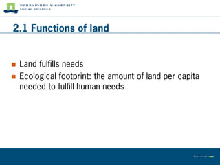
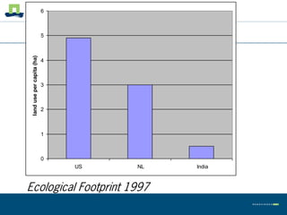
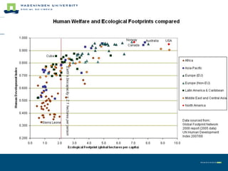
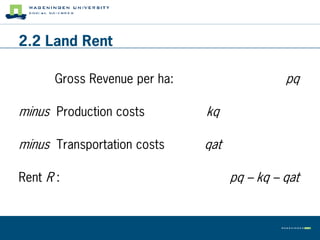
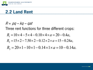
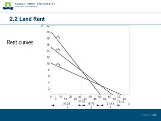
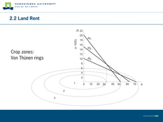
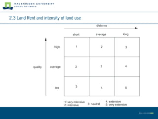
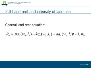
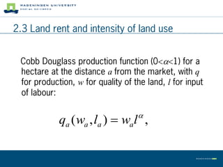
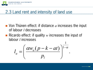
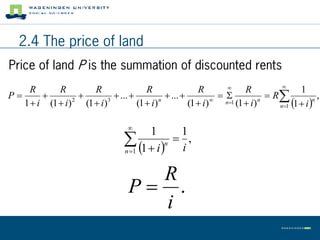
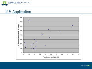
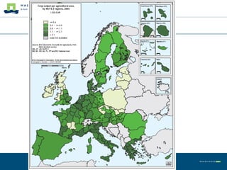
This document summarizes land use theory and economics. It discusses the functions of land including as a location for raw materials, capital goods, agriculture, and housing. Land rent theory is explained, with the rent determined by production, costs, and transportation costs. The quality and intensity of land use is related to distance from markets, according to Von Thünen, with the most intensive use closest to markets. Ricardo added that land quality also impacts intensity, with higher quality land used more intensively. Land prices are determined by discounting future rents. Applications show relationships between population density and productivity and fertilizer use.

1. Space and Economics
Chapter 2: Land use theory
Author
Wim Heijman (Wageningen, the Netherlands)
July 20, 2009

2. 2. Land use theory
 2.1 Functions of land
 2.2 Land rent
 2.3 Land rent and the intensity of land use
 2.4 The price of land

3. 2.1 Functions of land
 Location of raw materials
 Location and carrier of capital goods
 Input for agriculture
 Location and carrier for housing, recreation,
infrastructure

4. 2.1 Functions of land
 Land fulfills needs
 Ecological footprint: the amount of land per capita
needed to fulfill human needs

5. 6
land use per capita (ha) 5
4
3
2
1
0
US NL India
Ecological Footprint 1997

7. 2.1 Functions of land
 http://en.wikipedia.org/wiki/Ecological_footprint

8. 2.2 Land Rent
 Land rent: profit of a hectare
 Johann Heinrich Von Thünen (1783-1850): “The
Isolated State”
 Isotropic plane
 The quality of the soil is equal
 Transportation costs are proportional to the
distance

9. J.H. von Thünen
(1783-1850)

10. 2.2 Land Rent
Questions:
 Which crop is grown where?
 What explains the productivity of land and the intensity of
land use?
Solutions:
 Land will be used for the activity that generates the highest
possible rent.
 The closer to the market the higher the intensity of land use
and the more productive the land.

11. 2.2 Land Rent
Gross Revenue per ha: pq
minus Production costs kq
minus Transportation costs qat
Rent R : pq – kq – qat

12. 2.2 Land Rent
R = pq – kq – qat
Three rent functions for three different crops:
R1  10  4  5  4  0.10  4  a  20  0.4a,
R2  15  2  7.50  2  0.12  2  a  15  0.24a,
R3  20  1  10 1  0.14  1 a  10  0.14a.

13. 2.2 Land Rent
R 22
20
18
R1
Rent curves 16
R2
14
12
10 R3
8
6
4
2
0 10 20 30 40 50 60 70
5 15 25 35 45 55 65 75
31.25 71.43
31.25 18.75 21.43 a
1 2 3

14. 2.2 Land Rent
R 22
20
R1
18
(x 1000)
16
14 R2
Crop zones: 12
Von Thünen rings 10 R3
8
6
4
2
1 0 10 20 30 40 50 60 70 a
2
3

15. 2.3 Land Rent and intensity of land use
 David Ricardo (1772-1823), takes the differences
in land quality into account.
 According to Ricardo’s land rent theory the intensity
of land use (input of labour per ha) is the highest on
the land of the highest quality.

16. David Ricardo
(1772-1823)

17. 2.3 Land Rent and intensity of land use
distance
short average long
high 1 2 3
quality average 2 3 4
low 3 4 5
1: very intensive 4: extensive
2: intensive 3: neutral 5: very extensive

18. 2.3 Land rent and intensity of land use
General land rent equation:
Ra  pqa (wa , la )  kqa (wa , la )  aqa (wa , la )t  la pl ,

19. 2.3 Land rent and intensity of land use
Cobb Douglass production function (01) for a
hectare at the distance a from the market, with q
for production, w for quality of the land, l for input
of labour:

qa (wa , la )  wal ,

20. 2.3 Land rent and intensity of land use
 Von Thünen effect: if distance a increases the input
of labour l decreases
 Ricardo effect: if quality w increases the input of
labour l increases
1
 wa ( p  k  at )  1
la  
 
 .
 pl 

21. 2.4 The price of land
Price of land P is the summation of discounted rents
 
R R R R R R 1
P    ...   ...    R ,
n1   i 

1  i (1  i) (1  i)
2 3
(1  i) n
(1  i) n1 (1  i ) n 1
n

1 1
 1  i n  i ,
n 1
R
P .
i

22. 2.4 The price of land
Land speculation:
If agricultural land changes into residential land
then the price will increase. Speculators anticipate
that and buy agricultural land for relatively low
prices. They hope to sell it at high prices for
residential or industrial use in the future. If they are
successful they may gain high profits.
http://www.realestatejournal.com/columnists/houset
alk/20030530-barta.html

23. 2.5 Application
dI
I  I (X ), 0
dX
dY dY dY dI
Y  Y (I ),  0, so: Y  Y ( I ( X )), and   0,
dI dX dI dX

24. 2.5 Application
Table 2.3: Population density, productivity, and intensity of agriculture for a number of
European countries.
Country Population density X in Artificial fertilizer I Production Y per ha
(persons per ha, 1990) (kg per ha arable arable land ($, 1985)
land, 1990)
Belgium 3.298 470 1665
Denmark 1.197 243 711
Germany 2.275 520 1082
Finland 0.163 174 375
France 1.031 301 793
Greece 0.785 172 758
Hungary 1.142 142 598
Ireland 0.508 725 1976
Italy 1.960 160 1118
Yugoslavia 0.932 99 505
Netherlands 4.404 614 4716
Norway 0.138 234 549
Austria 0.931 199 1027
Portugal 1.073 84 335
Spain 0.780 98 404
United Kingdom 2.376 350 916
Sweden 0.208 113 415
Switzerland 1.687 413 2883
Source: United Nations (1994).

25. 2.5 Application
5000
4500
4000
Production per ha ($, 1985)
3500
3000
2500
2000
1500
1000
500
0
0 0.5 1 1.5 2 2.5 3 3.5 4 4.5 5
Population per ha (1990)

26. 2.5 Application
Y  789 X , (t - value of coefficien t in brackets; R  0.78).
2
( 7.76)

27. 2.5 Application
800
700
kg artificail fertilizer per ha (1990)
600
500
400
300
200
100
0
0 0.5 1 1.5 2 2.5 3 3.5 4 4.5 5
Population per ha (1990)

28. 2.5 Application
I  155.62 92.81 X , (t - values of coefficien ts in brackets; R 2  0.30).
( 2.48) ( 2.61)

29. 2.5 Application
Situation in 1830

30. 2.5 Application
Situation in 2000