Downloaded 150 times
![Kriging approach and terminology
Goovaerts, 1997: “All kriging estimators are but variants of the
basic linear regression estimator Z*(u) defined as
( ) ( ) [ ( ) ( )] ( )
Z m Z m
4
u
n
å=
- = -
u u u u
1
*
a
la a a .”
with
a u,u : location vectors for estimation point and one of the
neighboring data points, indexed by a
n(u): number of data points in local neighborhood used for
estimation of Z*(u)
( ), ( ): a m u m u expected values (means) of Z(u) and ( ) a Z u
(u) a l : kriging weight assigned to datum ( ) a z u for estimation
location u; same datum will receive different weight for
different estimation location
Z(u) is treated as a random field with a trend component, m(u),
and a residual component, R(u) = Z(u)- m(u). Kriging estimates
residual at u as weighted sum of residuals at surrounding data
points. Kriging weights, a l , are derived from covariance function
or semivariogram, which should characterize residual component.
Distinction between trend and residual somewhat arbitrary; varies
with scale.
Development here will follow that of Pierre Goovaerts, 1997,
Geostatistics for Natural Resources Evaluation, Oxford University
Press.](https://image.slidesharecdn.com/kriging-141216024725-conversion-gate02/85/Kriging-4-320.jpg)
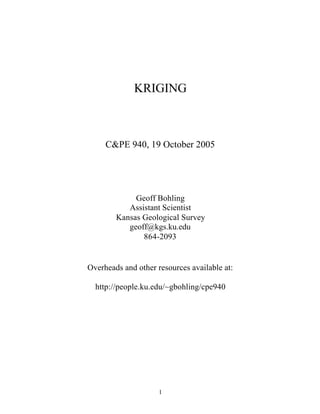
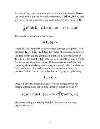
![Basics of Kriging
Again, the basic form of the kriging estimator is
( ) ( ) [ ( ) ( )] ( )
Z m Z m
6
u
n
å=
- = -
u u u u
1
*
a
la a a
The goal is to determine weights, a l , that minimize the variance of
the estimator
sE2 (u) = Var{Z *(u) - Z(u)}
under the unbiasedness constraint E{Z * (u)- Z (u)}= 0.
The random field (RF) Z(u) is decomposed into residual and trend
components, Z(u) = R(u) + m(u), with the residual component
treated as an RF with a stationary mean of 0 and a stationary
covariance (a function of lag, h, but not of position, u):
E{R(u)}= 0
Cov{R(u),R(u+ h)}= E{R(u)× R(u +h)}= CR (h)
The residual covariance function is generally derived from the
input semivariogram model, C (h) = C (0)-g (h) = Sill -g (h) R R .
Thus the semivariogram we feed to a kriging program should
represent the residual component of the variable.
The three main kriging variants, simple, ordinary, and kriging with
a trend, differ in their treatments of the trend component, m(u).](https://image.slidesharecdn.com/kriging-141216024725-conversion-gate02/85/Kriging-6-320.jpg)
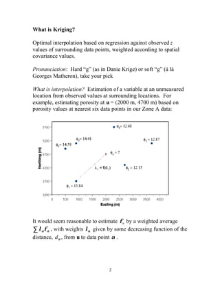
![Simple Kriging
For simple kriging, we assume that the trend component is a
constant and known mean, m(u) = m, so that
( ) ( ) [ ( ) ] ( )
n(u)
å SK (u)R ( u)
- R(u)= Ra SK
{ * (u)}+Var RSK { (u)}- 2Cov RSK
n(u)
å +CR (0)- 2 la
SK 1, ,
l - = a - a
= K å=
7
u
å=
= + u u
-
n
SK
ZSK u m Z m
1
*
a
la a .
This estimate is automatically unbiased, since E[Z( ) -m] = 0 a u , so
that [Z (u)] m [Z(u)] SK E * = = E . The estimation error Z (u) Z(u) SK * -
is a linear combination of random variables representing residuals
at the data points, a u , and the estimation point, u:
* (u)- Z(u)= ZSK
ZSK
[ * (u)-m]- [Z (u)-m]
= la
a=1
* (u)- R(u)
Using rules for the variance of a linear combination of random
variables, the error variance is then given by
sE
2 (u)= Var RSK
* (u),RSK { (u)}
SK (u)lb
n(u)
å
= la
SK (u)CR ua -ub ( )
b=1
a=1
SK (u)CR ua ( - u)
n(u)
å
a=1
To minimize the error variance, we take the derivative of the above
expression with respect to each of the kriging weights and set each
derivative to zero. This leads to the following system of equations:
( u
) ( u ) ( u u ) (u u) (u)
C C n R
n
R
1
b
b a b](https://image.slidesharecdn.com/kriging-141216024725-conversion-gate02/85/Kriging-7-320.jpg)
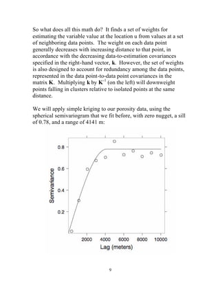
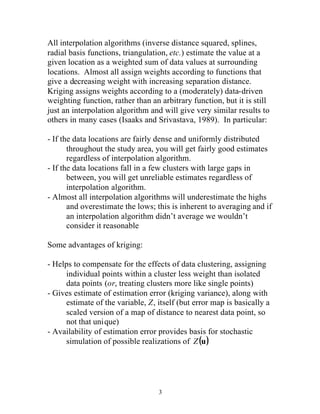
![Since we are using a spherical semivariogram, the covariance
function is given by
C(h) = C(0)-g (h) = 0.78× (1-1.5× (h 4141)+ 0.5× (h 4141)3 )
for separation distances, h, up to 4141 m, and 0 beyond that range.
The plot below shows the elements of the right-hand vector,
k = [0.38,0.56,0.32,0.49,0.46,0.37]T , obtained from plugging the
data-to-estimation-point distances into this covariance function:
The matrix of distances between the pairs of data points (rounded
to the nearest meter) is given by
Point 1 Point 2 Point 3 Point 4 Point 5 Point 6
Point 1 0 1897 3130 2441 1400 1265
Point 2 1897 0 1281 1456 1970 2280
Point 3 3130 1281 0 1523 2800 3206
Point 4 2441 1456 1523 0 1523 1970
Point 5 1400 1970 2800 1523 0 447
Point 6 1265 2280 3206 1970 447 0
10](https://image.slidesharecdn.com/kriging-141216024725-conversion-gate02/85/Kriging-10-320.jpg)
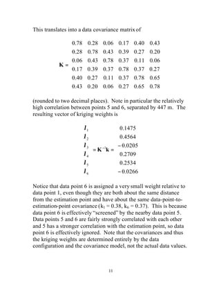
![The porosities at points 5 and 6 could in fact be very different and
this would have no influence on the kriging weights.
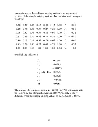
The mean porosity value for the 85 wells is 14.70%, and the
porosity values at the six example wells are 13.84%, 12.15%,
12.87%, 12.68%, 14.41%, and 14.59%. The estimated residual
from the mean at u is given by the dot product of the kriging
weights and the vector of residuals at the data points:
( )
- 0.86
ù
ú ú ú ú ú ú ú
é
- 2.55
-1.83
R u = ?¢Ra
[ 0.15 0.46 0.02 0.27 0.25 0.03 ] = -
1.87
12
- 2.01
- 0.28
- 0.10
û
ê ê ê ê ê ê ê
ë
= - -
Adding the mean back into this estimated residual gives an
estimated porosity of Zˆ(u) = R(u) + m = -1.87 +14.70 =12.83%.
Similarly, plugging the kriging weights and the vector k into the
expression for the estimation variance gives a variance of 0.238
(squared %). Given these two pieces of information, we can
represent the porosity at u = (2000 m, 4700 m) as a normal
distribution with a mean of 12.83% and a standard deviation of
0.49%. Note that, like the kriging weights, the variance estimate
depends entirely on the data configuration and the covariance
function, not on the data values themselves. The estimated kriging
variance would be the same regardless of whether the actual
porosity values in the neighborhood were very similar or highly
variable. The influence of the data values, through the fitting of
the semivariogram model, is quite indirect.](https://image.slidesharecdn.com/kriging-141216024725-conversion-gate02/85/Kriging-12-320.jpg)
![Ordinary Kriging
For ordinary kriging, rather than assuming that the mean is
constant over the entire domain, we assume that it is constant in
the local neighborhood of each estimation point, that is that
m(u ) = m(u) a for each nearby data value, ( ) a Z u , that we are using
to estimate Z(u). In this case, the kriging estimator can be written
( ) ( ) n
( )
= + l
( )[ ( ) -
( )] Z m Z m
u u u u u
=
1
a
( ) ( ) ( ) ( ) ( ) u u u (u)
= + é -
n n
u u
å å
u n
u
* u = å u u å u
=
= =
é - + = å=
s m la
E OK L
u
= - =
15
u
ù
Z m
úû
êë
å
= =
1 1
*
1
a
a
a
a a
a a
l l
and we filter the unknown local mean by requiring that the kriging
weights sum to 1, leading to an ordinary kriging estimator of
( )
( ) ( ) ( )
( )
( )
with 1
1 1
OK
n
OK
ZOK Z
a
a
a
la a l .
In order to minimize the error variance subject to the unit-sum
constraint on the weights, we actually set up the system minimize
the error variance plus an additional term involving a Lagrange
parameter, (u) OK m :
( ) ( ) ( ) ( )
ù
úû
êë
u
n
u u u
1
2 2 1
a
so that minimization with respect to the Lagrange parameter forces
the constraint to be obeyed:
( ) ( )
1 0
1
2
1
å=
u
L n
a
a l
m](https://image.slidesharecdn.com/kriging-141216024725-conversion-gate02/85/Kriging-15-320.jpg)
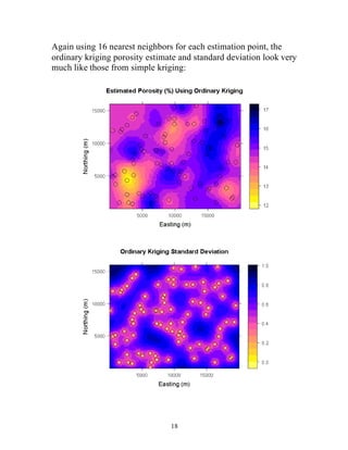

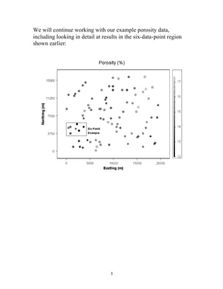
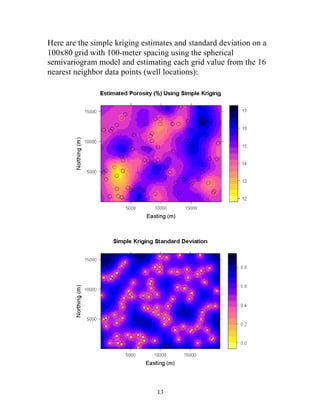
Kriging is an optimal interpolation technique that estimates values at unmeasured locations based on measured data from nearby locations. It assigns weights to surrounding data points based on their distances and spatial covariance, accounting for clustering of data points. Simple kriging assumes a known mean and estimates values as a weighted average of residuals from the mean at nearby locations, with weights chosen to minimize the estimation variance. The document provides an example of applying simple kriging to estimate porosity using six nearby data points.