The document outlines a training program for digital soil organic carbon mapping using regression-kriging, a spatial interpolation technique that integrates regression modeling with kriging. It details the workflow for mapping soil properties, including data preparation, model fitting using multiple linear regression, and assessing model validity through residual analysis and collinearity checks. The document culminates in predicting soil carbon values and generating raster outputs for visualization and analysis.

1. FAO- Global Soil
Partnership
Training on
Digital Soil Organic Carbon
Mapping
20-24 January 2018
Tehran/Iran
Yusuf YIGINI, PhD - FAO, Land and Water Division (CBL)
Guillermo Federico Olmedo, PhD - FAO, Land and Water Division (CBL)

2. Regression Kriging

3. REGRESSION KRIGING
Regression-kriging is a spatial interpolation
technique that combines a regression of the
dependent variable (target variable) on predictors
(i.e. the environmental covariates) with kriging of
the prediction residuals. In other words,
Regression-Kriging is a hybrid method that
combines either a simple or a multiple-linear
regression model with ordinary kriging of the
prediction residuals.

4. REGRESSION KRIGING
The modelled relationship between predictors and
target are summarized in regression equation,
which can then be applied to a different data set in
which the target values are unknown but the
predictor variables are known. The regression
equation predicts the value of the dependent
variable using a linear function of the independent
variables.

5. REGRESSION KRIGING

8. WORKFLOW
1/ The first step is to prepare a map showing the
spatial distribution of the sample locations and the
corresponding soil property information, e.g. soil
organic matter and environmental properties. The
first can be achieved as outlined in section Overlay
covariates and spatial data. The overlaying
operation can be performed in R, ArcGIS, SAGA GIS
or QGIS.

9. WORKFLOW
2/ The essential part of multiple regression analysis
is to build a regression model by using the
environmental predictors. After extracting the
values of explanatory maps and target variables
into the single table, we can now start fitting
multiple regression model using the table that
contains data from dependent variable and
predictors.

10. WORKFLOW
3/ In particular cases, stepwise multiple linear
regression (SMLR) can be used to eliminate
insignificant predictors. Stepwise multiple linear
regression (SMLR) usually selects predictors that
have the strongest linear correlations with the
target variable, which reflect the highest predictive
capacity.

11. WORKFLOW
4/ Kriging of the residuals (prediction errors): In
regression-kriging, the regression model detrends
the data, produces the residuals which we need to
krige and to be added to the regression model
predictions.

12. Interpret the key results
Regression analysis generates an equation to
describe the statistical relationship between one or
more predictor variables and the response variable.
he r-squared, p-values and coefficients that appear
in the output for linear regression analysis must
also be reviewed. Before accepting the result of a
linear regression it is important to evaluate its
suitability at explaining the data. One of the many
ways to do this is to visually examine the residuals.
If the model is appropriate, then the residual errors
should be random and normally distributed.

13. Interpret the key results
Rsq
R2 is the percentage of variation in the response
that is explained by the model. The higher the R2
Value, the better the model fits your data. R-
squared is always between 0% and 100%. R2
usually increases when additional predictors are
added in the model.

14. Interpret the key results
P Values
To determine whether the association between the
dependent and each predictor in the model is
statistically significant, compare the p-value for the
term to your significance level to assess the null
hypothesis. Usually, a significance level of 0.05
works well.

15. Interpret the key results
P-value ≤ significance level: The relationship is statistically
significant. If the p-value is less than or equal to the
significance level, we can conclude that there is a
statistically significant relationship between the dependent
variable and the predictor.
P-value > significance level: The relationship is not
statistically significant, If the p-value is greater than the
significance level, you cannot conclude that there is a
statistically significant relationship between the dependent
variable and the predictor. You may want to refit the model
without the predictor.

16. Interpret the key results
Residuals
We can plot the residuals which can help us determine
whether the model is adequate and meets the assumptions
of the analysis. If the model is appropriate, then the residual
errors should be random and normally distributed. We can
plot residuals versus fits to verify the assumption that the
residuals are randomly distributed and have constant
variance. Ideally, the points should fall randomly on both
sides of “0”, with no recognizable patterns in the points.

17. Interpret the key results
Residuals
The diagnostic plots for the model should be evaluated to
confirm if all the assumptions of linear regression are met.
After the above mentioned assumptions are validated, we
can proceed with making the prediction map using the
model with significant predictors.

18. Regression Kriging
## set working directory
setwd("C:/rk")
## Install required packages
install.packages("raster")
install.packages("car")
install.packages("rgdal")
install.packages("gstat")
install.packages("caret")
install.packages("reshape")
## Load required packages
library(raster)
library(car)
library(rgdal)
library(gstat)
library(caret)
library(reshape)
Step 1. Setting the working environment and installing/loading
required packages

19. Regression Kriging
# load data
dat <- read.csv("data/MKD_RegMatrix.csv")
dat$LCEE10 <- as.factor(dat$LCEE10)
dat$soilmap <- as.factor(dat$soilmap)
# explore the data structure
str(dat)
Step 2. Import Data

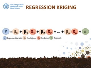
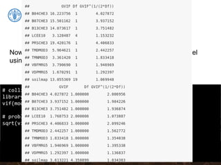
20. Regression Kriging
library(sp)
# Promote to spatialPointsDataFrame
coordinates(dat) <- ~ X + Y
class(dat)
## [1] "SpatialPointsDataFrame"
## attr(,"package")
## [1] "sp"
Since we will be working with spatial data we need to define
the coordinates for the imported data. Using the coordinates()
function from the sp package we can define the columns in the
data frame to refer to spatial coordinates—here the coordinates
are listed in columns X and Y.

21. CRS
SpatialPointsDataFrame structure is essentially the
same data frame, except that additional “spatial”
elements have been added or partitioned into slots.
Some important ones being the bounding box (sort of
like the spatial extent of the data), and the coordinate
reference system proj4string(), which we need to
define for the sample dataset. To define the CRS, we
must know where our data are from, and what was the
corresponding CRS used when recording the spatial
information in the field. For this data set the CRS used
was: WGS84 (EPSG:4326).

22. CRS
Please also note that, when working with spatial data,
it’s very important that the CRS (coordinate reference
system) of the point data and covariates are the same.
Now, we will define our CRS:
dat@proj4string <- CRS(projargs = "+init=epsg:4326")
dat@proj4string
## CRS arguments:
## +init=epsg:4326 +proj=longlat +datum=WGS84 +no_defs
## +ellps=WGS84 +towgs84=0,0,0

23. Covariates
Now we will import the covariates. When the covariate
layers are in common resolution and extent, rather
than working with individual rasters it is better to stack
them all into a single R object. We will use stack()
function from raster package. In this example we use
13 covariates from the GSOCMap Data Repository and
a rasterized version of the soil type map.

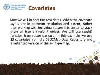
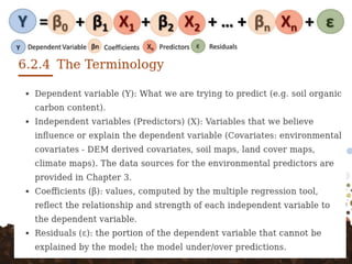
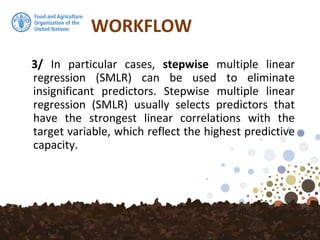
24. Covariates
library(raster)
# list all the itf files in the folder covs/
files <- list.files(path = "covs", pattern = "tif$",
full.names = TRUE)
# load all the tif files in one rasterStack object
covs <- stack(files)
# load the vectorial version of the soil map
soilmap <- shapefile("MK_soilmap_simple.shp")
# rasterize using the Symbol layer
soilmap@data$Symbol <- as.factor(soilmap@data$Symbol)
soilmap.r <- rasterize(x = soilmap, y = covs[[1]], field = "Symbol")

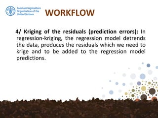
25. Covariates
# stack the soil map and the other covariates
covs <- stack(covs, soilmap.r)
# correct the name for layer 14
names(covs)[14] <- "soilmap"
# print the names of the 14 layers:
names(covs)
## [1] "B04CHE3" "B07CHE3" "B13CHE3" "B14CHE3" "DEMENV5" "LCEE10"
## [7] "PRSCHE3" "SLPMRG5" "TMDMOD3" "TMNMOD3" "TWIMRG5" "VBFMRG5"
## [13] "VDPMRG5" "soilmap"

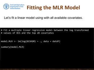
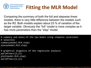
26. Fitting the MLR Model
datdf <- dat@data
datdf <- datdf[, c("OCSKGM", names(covs))]
It would be better to progress with a data frame of just the
data and covariates required for the modelling. In this case,
we will subset the columns SOC, the covariates and the the
spatial coordinates (X and Y).

27. Fitting the MLR Model
# Fit a multiple linear regression model between the log transformed
# values of OCS and the top 20 covariates
model.MLR <- lm(log(OCSKGM) ~ ., data = datdf)
summary(model.MLR)
Let’s fit a linear model using with all available covariates.

28. Fitting the MLR Model
# stepwise variable selection
model.MLR.step <- step(model.MLR, direction="both")
From the summary of our fitted model (model.MLR) above,
it seems only a few of the covariates are significant in
describing the spatial variation of the target variable. To
determine the most predictive model we can run a stepwise
regression using the step() function. With this function we
can also specify the mode of stepwise search, can be one
of “both”, “backward”, or “forward”.

29. Fitting the MLR Model
# summary and anova of the new model using stepwise covariates
# selection
summary(model.MLR.step)
anova(model.MLR.step)
# graphical diagnosis of the regression analysis
par(mfrow=c(2,2))
plot(model.MLR.step)
par(mfrow=c(1,1))
Comparing the summary of both the full and stepwise linear
models, there is very little difference between the models such
as the R2. Both models explain about 23 % of variation of the
target variable. Obviously the “full” model is more complex as it
has more parameters than the “step” model.

30. Fitting the MLR Model
# graphical diagnosis of the regression analysis
par(mfrow=c(2,2))
plot(model.MLR.step)
Now we can evaluate the test statistics of the calibration model
using the goof() function from the “ithir” package.

31. Fitting the MLR Model
# graphical diagnosis of the regression analysis
par(mfrow=c(2,2))
plot(model.MLR.step)
Now we can evaluate the test statistics of the calibration model
using the goof() function from the “ithir” package.

32. Collinearity
# collinearity test using variance inflation factors
library(car)
vif(model.MLR.step)
# problematic covariates should have sqrt(VIF) > 2
sqrt(vif(model.MLR.step))
Now we can evaluate the test statistics of the calibration model
using the goof() function from the “ithir” package.

33. Collinearity
# collinearity test using variance inflation factors
library(car)
vif(model.MLR.step)
# problematic covariates should have sqrt(VIF) > 2
sqrt(vif(model.MLR.step))
Now we can evaluate the test statistics of the calibration model
using the goof() function from the “ithir” package.

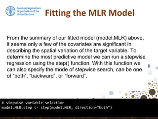
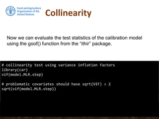
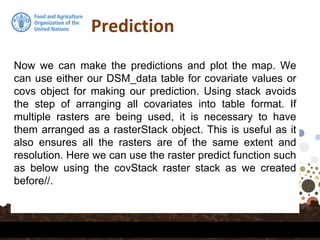
34. Collinearity
# Removing B07CHE3 from the stepwise model:
model.MLR.step <- update(model.MLR.step, . ~ . - B07CHE3)
# Test the vif again:
sqrt(vif(model.MLR.step))
# summary of the new model using stepwise covariates selection
summary(model.MLR.step)
collinear: Temperature seasonality at 1 km (B04CHE3) and
Temperature Annual Range [°C] at 1 km (B07CHE3)

35. Prediction
Now we can make the predictions and plot the map. We
can use either our DSM_data table for covariate values or
covs object for making our prediction. Using stack avoids
the step of arranging all covariates into table format. If
multiple rasters are being used, it is necessary to have
them arranged as a rasterStack object. This is useful as it
also ensures all the rasters are of the same extent and
resolution. Here we can use the raster predict function such
as below using the covStack raster stack as we created
before//.

36. Prediction
# Project point data.
dat <- spTransform(dat, CRS("+init=epsg:6204"))
# project covariates to VN-2000 UTM 48N
covs <- projectRaster(covs, crs = CRS("+init=epsg:6204"),
method='ngb')
covs$LCEE10 <- as.factor(covs$LCEE10)
covs$soilmap <- as.factor(covs$soilmap)

37. # Promote covariates to spatial grid dataframe. Takes some time and
# a lot of memory!
covs.sp <- as(covs, "SpatialGridDataFrame")
covs.sp$LCEE10 <- as.factor(covs.sp$LCEE10)
covs.sp$soilmap <- as.factor(covs.sp$soilmap)
Prediction

38. ### RK model
library(automap)
## Run regression kriging prediction. This step can take hours...!
OCS.krige <- autoKrige(formula =
as.formula(model.MLR.step$call$formula),
input_data = dat,
new_data = covs.sp,
verbose = TRUE,
block = c(1000, 1000))
OCS.krige
## Checking if any bins have less than 5 points, merging bins when
necessary...
##
## Selected:
## model psill range
## 1 Nug 0.19748915 0.00
## 2 Sph 0.04812862 6982.47
##
...
Prediction

39. ## Convert prediction and standard deviation to rasters
#
# And back-tansform the vlaues
RKprediction <- exp(raster(OCS.krige$krige_output[1]))
RKpredsd <- exp(raster(OCS.krige$krige_output[3]))
plot(RKprediction)
Prediction

40. ## Convert prediction and standard deviation to rasters
#
# And back-tansform the vlaues
RKprediction <- exp(raster(OCS.krige$krige_output[1]))
RKpredsd <- exp(raster(OCS.krige$krige_output[3]))
plot(RKprediction)
Prediction

41. ## Convert prediction and standard deviation to rasters
#
# And back-tansform the vlaues
RKprediction <- exp(raster(OCS.krige$krige_output[1]))
RKpredsd <- exp(raster(OCS.krige$krige_output[3]))
plot(RKprediction)
plot(RKpredsd)
Standard Dev

42. ## Convert prediction and standard deviation to rasters
#
# And back-tansform the vlaues
RKprediction <- exp(raster(OCS.krige$krige_output[1]))
RKpredsd <- exp(raster(OCS.krige$krige_output[3]))
plot(RKprediction)
plot(RKpredsd)
Standard Dev

43. ## Convert prediction and standard deviation to rasters
#
# And back-tansform the vlaues
RKprediction <- exp(raster(OCS.krige$krige_output[1]))
RKpredsd <- exp(raster(OCS.krige$krige_output[3]))
plot(RKprediction)
plot(RKpredsd)

44. ## Save results as tif files
writeRaster(RKprediction, filename = "results/MKD_OCSKGM_RK.tif",
overwrite = TRUE)
writeRaster(RKpredsd, filename = "results/MKD_OCSKGM_RKpredsd.tif",
overwrite = TRUE)
# save the model
saveRDS(model.MLR.step, file="results/RKmodel.Rds")
Final bits...