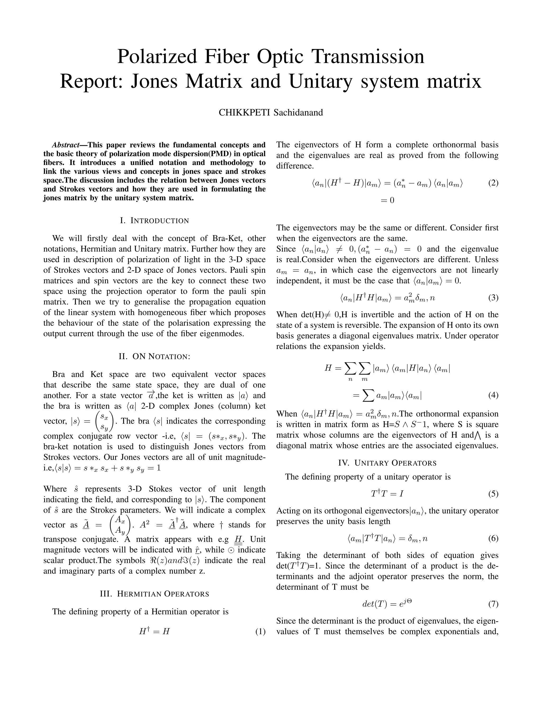
SlideShare a Scribd company logo
Polarized Fiber Optic Transmission
Report: Jones Matrix and Unitary system matrix
CHIKKPETI Sachidanand
Abstract—This paper reviews the fundamental concepts and
the basic theory of polarization mode dispersion(PMD) in optical
fibers. It introduces a unified notation and methodology to
link the various views and concepts in jones space and strokes
space.The discussion includes the relation between Jones vectors
and Strokes vectors and how they are used in formulating the
jones matrix by the unitary system matrix.
I. INTRODUCTION
We will firstly deal with the concept of Bra-Ket, other
notations, Hermitian and Unitary matrix. Further how they are
used in description of polarization of light in the 3-D space
of Strokes vectors and 2-D space of Jones vectors. Pauli spin
matrices and spin vectors are the key to connect these two
space using the projection operator to form the pauli spin
matrix. Then we try to generalise the propagation equation
of the linear system with homogeneous fiber which proposes
the behaviour of the state of the polarisation expressing the
output current through the use of the fiber eigenmodes.
II. ON NOTATION:
Bra and Ket space are two equivalent vector spaces
that describe the same state space, they are dual of one
another. For a state vector −
→
a ,the ket is written as |a⟩ and
the bra is written as ⟨a| 2-D complex Jones (column) ket
vector, |s⟩ =

sx
sy

. The bra ⟨s| indicates the corresponding
complex conjugate row vector -i.e, ⟨s| = (s∗x, s∗y). The
bra-ket notation is used to distinguish Jones vectors from
Strokes vectors. Our Jones vectors are all of unit magnitude-
i.e,⟨s|s⟩ = s ∗x sx + s ∗y sy = 1
Where ŝ represents 3-D Stokes vector of unit length
indicating the field, and corresponding to |s⟩. The component
of ŝ are the Strokes parameters. We will indicate a complex
vector as à =

Ax
Ay

. A2
= Ã
†
Ã, where † stands for
transpose conjugate. A matrix appears with e.g H. Unit
magnitude vectors will be indicated with r̂, while ⊙ indicate
scalar product.The symbols ℜ(z)andℑ(z) indicate the real
and imaginary parts of a complex number z.
III. HERMITIAN OPERATORS
The defining property of a Hermitian operator is
H†
= H (1)
The eigenvectors of H form a complete orthonormal basis
and the eigenvalues are real as proved from the following
difference.
⟨an|(H†
− H)|am⟩ = (a∗
n − am) ⟨an|am⟩ (2)
= 0
The eigenvectors may be the same or different. Consider first
when the eigenvectors are the same.
Since ⟨an|an⟩ ̸= 0, (a∗
n − an) = 0 and the eigenvalue
is real.Consider when the eigenvectors are different. Unless
am = an, in which case the eigenvectors are not linearly
independent, it must be the case that ⟨an|am⟩ = 0.
⟨an|H†
H|am⟩ = a2
mδm, n (3)
When det(H)̸= 0,H is invertible and the action of H on the
state of a system is reversible. The expansion of H onto its own
basis generates a diagonal eigenvalues matrix. Under operator
relations the expansion yields.
H =
X
n
X
m
|am⟩ ⟨am|H|an⟩ ⟨am|
=
X
am|am⟩⟨am| (4)
When ⟨an|H†
H|am⟩ = a2
mδm, n.The orthonormal expansion
is written in matrix form as H=S ∧ S−
1, where S is square
matrix whose columns are the eigenvectors of H and
V
is a
diagonal matrix whose entries are the associated eigenvalues.
IV. UNITARY OPERATORS
The defining property of a unitary operator is
T†
T = I (5)
Acting on its orthogonal eigenvectors|an⟩, the unitary operator
preserves the unity basis length
⟨am|T†
T|an⟩ = δm, n (6)
Taking the determinant of both sides of equation gives
det(T†
T)=1. Since the determinant of a product is the de-
terminants and the adjoint operator preserves the norm, the
determinant of T must be
det(T) = ejΘ
(7)
Since the determinant is the product of eigenvalues, the eigen-
values of T must themselves be complex exponentials and,
accounting for(7), they must have unity magnitude. Therefore
T acting on an eigenvector yields
T|an⟩ = ejαn
|an⟩ (8)
The eigenvalues of T lie on the unit circle in the complex
plane. A special form of T exists where the determinant is
unity. This special form is denoted U and is characterized
by det(U)=+1. To transform from T to U,the common phase
factorβ = exp(jΘ/N) must be extracted from each eigenvalue
of T, when N is the dimensionality of the operator. The T and
U forms are thereby related:
T = ejβ
U (9)
It should be noted that when det(U) = -1,a reflection is present
along an odd number of axes in the basis set of U is
U|an⟩ = e−jϕn
|an⟩ (10)
U expands on its own basis set in the same way H expands
(10).
U =
X
m
e−
jϕm|am⟩⟨am| (11)
This orthonormal expansion has the matrix analogue of U =
Sexp(−j∧)S−
1, where the diagonal matrix is exp(−j∧)=






e−
jϕ1
e−
jϕ2
.
.
e−
jϕN






(12)
Consider as a 2 × 2 unitary complex matrix U can always
be written as U = eiϕ

u1 u2
−u2
∗
u1∗

where the complex
numbers u1 and u2 satisfy |u1|2
+ |u2|2
=1, and ϕ is real.
V. CONNECTION BETWEEN HERMITIAN AND UNITARY
MATRICES:
The connection between Hermitian and Unitary operators is
quite intimate. The eigenvalues of H lies on the real number
line, while those of U lie on the unit circle in the complex
plane. Multiplying the eigenvalues of H by-j and taking the
exponential,one can construct the eigenvalues of U. Note that
the eigenvalues of U are cyclic, so only the real number line
modulo 2Π is significant.Based on the operator expansions of
the preceding sections one has
H = S ∧H S−1
(13)
U = Re−
j∧mR−1
(14)
Since in general exp(S ∧ S−1
)=Sexp(∧)S−1
, the H and U
operators may be connected as
U = e−jH
=⇒ Se−
j∧U S−1
= Se−
j∧HS−1
(15)
For every Hermitian operator H there is a associated unitary
operator U that shares the same basis set and has eigenvalues
related through the complex exponential.
VI. JONES AND STOKES SPACES:-
The preceding paper will concentrate on the study of
polarization which forms the connection between Jones and
Stokes space. From the tangential relation between the electric
fields, the Jones vector can be written in normalized form:
E = E0ejΘ

cosχ
sinχejϕ

(16)
where E0 is real. There are the polar angles in above equa-
tion(16) χandϕ.The phase exp(jΘ) is lost on conversion
to Stokes space. The jones vectors two orthogonal state of
polarisation are combined together or projected to form the
Paulis spin matrices which are further as discussed below.
A. Pauli Spin Matrices:-
The Pauli spin matrices connect Jones to Stokes space
through the projection measurements of the preceding section.
The identity Pauli matrix is
σ0 =

1 0
0 1

(17)
The Pauli spin matrices are
σ1 =

1 0
0 −1

; σ2 =

0 1
1 0

; σ3 =

0 −j
j 0

; (18)
The spin matrices are both Hermitian and Unitary:
σ†
k = σk and σ†
kσk = I (19)
The determinants of the spin matrices are −1 and the traces
zero:
det(σk) = −1 and Tr(σk = 0 (20)
A spin matrix multiplied by itself yields
σkσk = I (21)
and multiplied by other matrices gives
σiσj = −σiσj = jσj (22)
Each Stokes coordinate of a polarization state|s⟩ is calculated
by inserting the associated Pauli matrix into the inner product
⟨s|.|s⟩. The individual Stokes coordinates are
sk = ⟨s|σk|s⟩ (23)
Since the spin matrices are Hermitian, the Stokes coordinates
sK are real, signed quantities, since det(σk) = −1 and the
Jones vector |s⟩ is assumed to be normalised, sk is bounded
by −1 ≤ sk ≤ +1. The norm of ŝ is unity, |s| = 1,
B. The Pauli Spin Matrices and its bilateral connection be-
tween the Jones and Stokes Vectors:-
The pauli spin vector condenses further the notation of (23).
The spin vector is defined as
−
→
σ =


σ1
σ2
σ3

 (24)
where −
→
σ is a vector of matrices. The vector of Stokes
coordinates ŝ is derived from the Jones vector |s⟩ using the
spin vector: 

s1
s2
s3

 =


⟨s|σ1|s⟩
⟨s|σ2|s⟩
⟨s|σ3|s⟩

 (25)
More concisely,
ŝ = ⟨s|−
→
σ |s⟩ (26)
The most compact map of Jones vectors to Stokes vectors.
Then the above formulated equation is equated by its vec-
tor form like sx, sy


1 0
0 1
 
sx
sy

, for all stokes vectors
,Then we get the following form of stokes vectors equation.
s0 = |sx|2
+ |sy|2
s1 = |sx|2
− |sy|2
s2 = 2ℜ|s∗
xsy|
s3 = 2ℑ|s∗
xsy|
and now by taking the projection combination of the bra-ket
vector of |s⟩⟨s| we get the following matrix
=

 |sx|2
  sxsy
∗

 sx
∗
sy   |sx|2


incorporating the stokes vectors given above into the following
matrix, First, observe that the spin vector behaves both as
3 × 1 vector and as a 2 × 2 matrix, depending on the
context(25). Above shows the spin vector acting as a 3 × 1
vector. Alternatively, the dot product of ŝ with the spin vector
yields.
ŝ.−
→
σ = 1/2(s0σ0+s1σ1+s2σ2+s3σ3) = 1/2

s0 + s1 s2 − js3
s2 + js3 s0 − s1

(27)
ŝ.−
→
σ in this case is a 2 × 2 Jones matrix and, since the
coefficients sk are real,ŝ.−
→
σ is Hermitian: (ŝ.−
→
σ )†
= (ŝ.−
→
σ ).
The trace operation connects the projection with its inner
product: Tr(|s⟩⟨s|) = ⟨s|s⟩.Since the trace of each Pauli
matrix is zero it is also true that Tr(ŝ.−
→
σ ) = 0 .For a
normalized state vector such that ⟨s|s⟩ = 1, one can construct
the projector for ket |s⟩ in terms of the spin vector:
|s⟩⟨s| = 1/2(I + ŝ.−
→
σ ) (28)
Subsequent multiplication on the right by |s⟩ generates the
eigenvalue equation
ŝ.−
→
σ |s⟩ = |s⟩ (29)
This is the most compact way to map Stokes vectors to Jones
vectors. The eigenvector of ŝ.−
→
σ associated with eigenvalue
+1 generates the Jones vector |s⟩ from Stokes vector ŝ.
VII. THE PROPAGATION EQUATION:
Consider a linear and Homogeneous fiber which is time
invariant and frequency dependent system as shown in the
below figure:
. By the linear system approach in the frequency domain
equation is given as
−
→
E (z, ω) =
−
→
T (z, ω)
−
→
E (0, ω) (30)
The optical fiber can be read as a linear time invariant system
with frequency response
T̃(ω) = e− α
2 z
e−jβ(ω)z
the first term in the equation produces the loses in the fiber
where as the second gives intensity/energy of the system.
By applying the partial differential with respect to the ’z’ for
the whole equation we get
∂
−
→
E
∂z
(z, ω) = −
α
2
−
→
E (z, ω) − jβ(z, ω)
−
→
E (z, ω)
Where α
2 is present always due to the attenuation of the signal
in linear system. By the formulation of the birefringence axes
the wave travel with different propagation constants the x and
y axes are two rays travelling in z axes, x,y independent plane
wave travel through fiber experiences the different propagation
constant due to birefringence axes as given in figure:
.
Considering the diagonal case of the birefringence

βxx 0
0 βyy

by the common propagation β
∆
= βxx + βyy
and the difference propagation constant ∆β
∆
= βxx −βyy then
by degenerate case the vectorial linear Schroedinger equation
in polarization is given by the following
∂
−
→
E (z, ω)
∂z
= −
α
2
−
→
E (z, ω)−j
β
2
(ω)σ0
−
→
E (z, ω)−j
∆β
2
(ω)σ1
−
→
A(z, ω)
(31)
We are interested in the propagation of an optical field along
single mode optical fibers (SMF),we will deal with a general
linear optical system.
Let’s begin with the frequency domain description of the
complex field envelop along a linear loseless optical system
with possibly z-varying characteristics the equation given in
(30)
e
E(z, ω) = T(z, ω) e
E(0, ω)
where T is the input/output system matrix, from the input
(z = 0) to the point at coordinate z. Such matrix is known as
the Jones matrix of the system. Matrix T is unitary because of
the lossless requirement, i.e, T−1
= T†1
. This comes from the
fact that E2
(z, ω) = e
E(z, ω)
†
e
E(z, ω) is constant in z, which
by(30) implies T†
T is constant in z, and equals its value at
z=0, i.e. the identity matrix because a zero length fiber does
not alter the field. Properties of unitary and other matrices
widely used in this paper are summarized above. Taking the
derivative with respect to z of both sides of(30) gives.
∂ e
E(z, ω)
∂z
=
∂T(z, ω)
∂z
e
E(0, ω) (32)
and inverting(30) to express e
E(0, ω) in (32) which is always
possible except for the ideal polarizers gives
∂ e
E(z, ω)
∂z
= M(z, ω) e
E(0, ω) (33)
where
M(z, ω)
∆
=
∂T(z, ω)
∂z
T−1
(z, ω) (34)
is the local propagation matrix at coordinate z. The global
matrix T is thus the unique solution to the matrix equation.
∂T(z, ω)
∂z
= M(z, ω)T(z, ω), T(0, ω) = I (35)
Matrix M is skew-hermitian. In fact from(18) and its conjugate
transpose we get:
0 =
∂| e
E(z, ω)|2
∂z
=
∂ e
E
†
∂z
e
E + e
E
† ∂ e
E
∂z
(36)
= e
E
†
M† e
E + e
E
†
M e
E
= e
E
†
(M†
+ M) e
E
which is true for every e
E, hence it must be: M†
= −M. The
eigenmodes of M(z, ω) are called the local birefringence axes
of the system. Using the results in unitary matrix, we spec-
trally decompose M using the unitary matrix L
∆
= [L̂, ˆ
L0]of
its orthonormal birefringence axes, and its associated purely
imaginary eigenvalues −iβ, −iβ2
, being the propagation con-
stants β(z, ω) and β(z, ω) positive numbers, as:
M(z, ω) = −L(z, ω)

iβ(z, ω) 0
0 iβ0(z, ω)

L†
(z, ω)
(37)
and we labelled the two eigenvalues such that the birefringence
strength ∆β(z, ω)
∆
= β − β0 is positive at the frequency.
This amounts to assuming that the first axis L̂ has a lower
propagation speed than the other. We call it the slow
birefringence axis as shown in the figure.
. It is known from system theory that the matrix solution of
(35) satisfies:
det(T(z, ω)) = e
R z
0
T r[M(ζ,ω)]dζ
= e−i
R z
0
(β(ζ,ω)+β0(ζ,ω))dζ
(38)
being Tr(.) is the trace operator, which verifies that the
determinant of T has unity magnitude. It is also known that if
matrices M(z, ω)and
R z
0
M(ζ, ω)dζ commute for all z, then
the Jones matrix T, solution of (35), has the matrix exponential
form:
T(z, ω) = e
R z
0
M(ζ,ω)dζ
T(0, ω) = e
R z
0
M(ζ,ω)dζ
(39)
This is clearly the case when the birefringence axes do not
vary in z, i.e. L(z, ω) = L(ω), which corresponds to a z-
homogeneous fiber which we call a generalized polarization
maintaining fiber(GPMF) as in below figure. In such case
TGP MF
(z, ω) = L(ω)

ei
R z
0
β(ζ,ω)dζ
0
0 ei
R z
0
β0(ζ,ω)dζ

L†
(ω)
(40)
i.e, the global eigenmodes coincide with the birefringence
axes.
. However commercial SMFs are typically markedly z-
homogeneous, due to both the fabrication process and local
stresses in the installed cables, and do not satisfy(40)
. In the general (z, ω)- varying case, we can use the properties
of unitary matrices to spectrally decompose the global matrix
T in terms of its unit eigenvalues e−iϕs
.e−iϕf
and of their
associated unit eigenvectors B̂s, ˆ
Bf , as:
T = B

eiϕs
0
0 eiϕf

B†
(41)
where B
∆
= [B̂s, B̂s], and where we defined the common phase
ϕ = (ϕs + ϕf )/2, the differential phase ∆ϕ = (ϕs − ϕf ),
which is positive at the reference frequency, and introduced
the unitary matrix.
U
∆
= B

ei∆ϕ/2
0
0 ei∆ϕ/2

B†
= e
i ∆ϕ
2 B


1 0
0 −1

B†
(42)
which has unit determinant: det[U] = 1. all quantities in
(41)and (42) depends on both z and ω. The second equality
in (42) comes from the definition of the matrix exponential:
e
i ∆ϕ
2 B


1 0
0 −1

B†
∆
= Σ∞
k=0
(−i∆ϕ/2)k
k! {B

1 0
0 −1

B†
}k
by realizing that
{B

1 0
0 −1

B†
}k
= B

1 0
0 −1
k
B†
so that
e
−i
∆ϕ
2
B


1 0
0 −1

B†
= Be
−i
∆ϕ
2


1 0
0 −1


B†
.
[B−
→
σ B†
] = B−
→
σ1B†
B−
→
σ2B†
B−
→
σ3B†
......B−
→
σkB†
= B−
→
σ kB†
= B

1 0
0 (−1)k

B†
and the matrix exponential of a diagonal matrix is the diagonal
matrix whose entries are the exponentials of the entries in the
original matrix.
To make further progress, it is convenient to write explicitly B
in terms of the Stokes unit vector b̂ = [b1.b2, b3]T
associated
with the slow eigenmode B̂s. The Stokes representation of
SOP vectors is introduced in Paulis matrix. Using the repre-
sentation to build B starting from b̂, we obtain
Bσ1B†
=

b1 (b2 − ib3)
(b2 + ib3) −b1

= b̂
K
σ (43)
where σ1, i=1,2,3 are Pauli matrices, which are introduced
in above equation with there properties. The symbols σ =
[σ1, σ2, σ3]T
stands for the formal 3×1 vector whose compo-
nents are the Pauli matrices 1,2,3,so that the scalar products
v⊙σ with a 3×1 vector v is shorthand notation for Σ3
i=1viσi,
and represents a matrix. When the above equation get evalu-
ated with the equation(31) we get the PMD(Polarisation mode
dispersion)equation. We will see that the decomposition of
Jones system matrices on the basis of the Pauli matrices is a
key tool, enabling significant analytical advancements.
From(42) we can now compactly express U as a matrix
exponential as
U = e−i ∆
ϕ 2(b̂⊙σ)
(44)
and, using the method of Exponential Matrix Expansion by
Cayley- Hamilton theorem, we can rewrite U explicitly as:
U = cos(
∆
ϕ
2)σ0 − isin(
∆
ϕ
2)(b̂ ⊙ σ) (45)
VIII. REFERENCE
• Armando Vannucci, “ Polarized Fiber Optic Transmission
Notes”
• Alberto Bononi and Armando Vannucci, “PMD: a Math
Primer”
• J. P. Gordon and H. Kogelnik, “PMD fundamentals:
Polarization mode dispersion in optical fibers”
• Polarization Optics in Telecommunications by Jay N.
Damask
• Handling Polarized light by Mark Shtaif
https://www.eng.tau.ac.il/ shtaif/PolarizationClass.pdf
• https://www.wikipedia.com

More Related Content

What's hot

01 basic principles of ultrasound & basic term
01 basic principles of ultrasound & basic term01 basic principles of ultrasound & basic term
01 basic principles of ultrasound & basic termJuan Alcatruz
 
computed Tomography
computed Tomographycomputed Tomography
Optics part i
Optics   part iOptics   part i
Optics part i
Solo Hermelin
 
Transducers 2020
Transducers 2020Transducers 2020
Transducers 2020
sandileHLATSHWAYO3
 
RADIOLOGIA STANDARD E PATOLOGICA DEL BACINO
RADIOLOGIA STANDARD E PATOLOGICA DEL BACINORADIOLOGIA STANDARD E PATOLOGICA DEL BACINO
RADIOLOGIA STANDARD E PATOLOGICA DEL BACINO
Andrea Zattin
 
P T C
P T CP T C
P T C
Stef C
 
Peripheral arterial doppler
Peripheral  arterial dopplerPeripheral  arterial doppler
Peripheral arterial doppler
Dr. Mohit Goel
 
Benign bone tumors
Benign bone tumorsBenign bone tumors
Benign bone tumors
suriyaprakash nagarajan
 
Evidence-based gallbladder diseases
Evidence-based gallbladder diseasesEvidence-based gallbladder diseases
Evidence-based gallbladder diseases
Suchanar Rungrojanarak
 
Metal-Semiconductor Contact
Metal-Semiconductor ContactMetal-Semiconductor Contact
Metal-Semiconductor Contact
RCC Institute of Information Technology
 
CT perfusion physics and its application in Neuroimaging
CT perfusion physics and its application in NeuroimagingCT perfusion physics and its application in Neuroimaging
CT perfusion physics and its application in Neuroimaging
Dr.Suhas Basavaiah
 
Role of Imaging in Male Infertility
Role of Imaging in Male InfertilityRole of Imaging in Male Infertility
Role of Imaging in Male Infertility
Niranjan Chavan
 
20 peripheral arterial triplex ultrasound artifact pitfalls dr ahmed esawy
20 peripheral arterial triplex ultrasound  artifact pitfalls dr ahmed esawy20 peripheral arterial triplex ultrasound  artifact pitfalls dr ahmed esawy
20 peripheral arterial triplex ultrasound artifact pitfalls dr ahmed esawy
AHMED ESAWY
 
Role of medical imaging in management of arteriovenous fistula Dr. Muhammad B...
Role of medical imaging in management of arteriovenous fistula Dr. Muhammad B...Role of medical imaging in management of arteriovenous fistula Dr. Muhammad B...
Role of medical imaging in management of arteriovenous fistula Dr. Muhammad B...
Dr. Muhammad Bin Zulfiqar
 
Presentation1.pptx, radiological imaging of lower limb ischemia.
Presentation1.pptx, radiological imaging of lower limb ischemia.Presentation1.pptx, radiological imaging of lower limb ischemia.
Presentation1.pptx, radiological imaging of lower limb ischemia.Abdellah Nazeer
 
lecture5.ppt
lecture5.pptlecture5.ppt
lecture5.ppt
ssuserb4d806
 
ultrasound transducers and resolution
ultrasound transducers and resolutionultrasound transducers and resolution
ultrasound transducers and resolutionVallabhaneni Bhupal
 
Emergency CT: Updates
Emergency CT: UpdatesEmergency CT: Updates
Emergency CT: Updates
Rathachai Kaewlai
 
Ultrasound Elastography
Ultrasound Elastography Ultrasound Elastography
Ultrasound Elastography
Sahil Chaudhry
 

What's hot (20)

01 basic principles of ultrasound & basic term
01 basic principles of ultrasound & basic term01 basic principles of ultrasound & basic term
01 basic principles of ultrasound & basic term
 
computed Tomography
computed Tomographycomputed Tomography
computed Tomography
 
Optics part i
Optics   part iOptics   part i
Optics part i
 
Transducers 2020
Transducers 2020Transducers 2020
Transducers 2020
 
RADIOLOGIA STANDARD E PATOLOGICA DEL BACINO
RADIOLOGIA STANDARD E PATOLOGICA DEL BACINORADIOLOGIA STANDARD E PATOLOGICA DEL BACINO
RADIOLOGIA STANDARD E PATOLOGICA DEL BACINO
 
P T C
P T CP T C
P T C
 
Peripheral arterial doppler
Peripheral  arterial dopplerPeripheral  arterial doppler
Peripheral arterial doppler
 
Benign bone tumors
Benign bone tumorsBenign bone tumors
Benign bone tumors
 
Evidence-based gallbladder diseases
Evidence-based gallbladder diseasesEvidence-based gallbladder diseases
Evidence-based gallbladder diseases
 
Metal-Semiconductor Contact
Metal-Semiconductor ContactMetal-Semiconductor Contact
Metal-Semiconductor Contact
 
CT perfusion physics and its application in Neuroimaging
CT perfusion physics and its application in NeuroimagingCT perfusion physics and its application in Neuroimaging
CT perfusion physics and its application in Neuroimaging
 
Physics basic
Physics basicPhysics basic
Physics basic
 
Role of Imaging in Male Infertility
Role of Imaging in Male InfertilityRole of Imaging in Male Infertility
Role of Imaging in Male Infertility
 
20 peripheral arterial triplex ultrasound artifact pitfalls dr ahmed esawy
20 peripheral arterial triplex ultrasound  artifact pitfalls dr ahmed esawy20 peripheral arterial triplex ultrasound  artifact pitfalls dr ahmed esawy
20 peripheral arterial triplex ultrasound artifact pitfalls dr ahmed esawy
 
Role of medical imaging in management of arteriovenous fistula Dr. Muhammad B...
Role of medical imaging in management of arteriovenous fistula Dr. Muhammad B...Role of medical imaging in management of arteriovenous fistula Dr. Muhammad B...
Role of medical imaging in management of arteriovenous fistula Dr. Muhammad B...
 
Presentation1.pptx, radiological imaging of lower limb ischemia.
Presentation1.pptx, radiological imaging of lower limb ischemia.Presentation1.pptx, radiological imaging of lower limb ischemia.
Presentation1.pptx, radiological imaging of lower limb ischemia.
 
lecture5.ppt
lecture5.pptlecture5.ppt
lecture5.ppt
 
ultrasound transducers and resolution
ultrasound transducers and resolutionultrasound transducers and resolution
ultrasound transducers and resolution
 
Emergency CT: Updates
Emergency CT: UpdatesEmergency CT: Updates
Emergency CT: Updates
 
Ultrasound Elastography
Ultrasound Elastography Ultrasound Elastography
Ultrasound Elastography
 

Similar to Jones matrix formulation by the unitary matrix

Proportional and decentralized rule mcst games
Proportional and decentralized rule mcst gamesProportional and decentralized rule mcst games
Proportional and decentralized rule mcst gamesvinnief
 
M.Sc. Phy SII UIV Quantum Mechanics
M.Sc. Phy SII UIV Quantum MechanicsM.Sc. Phy SII UIV Quantum Mechanics
M.Sc. Phy SII UIV Quantum Mechanics
Pankaj Nagpure, Shri Shivaji Science College, Amravati
 
About Modelling of the Gravitational Fields
About Modelling of the Gravitational FieldsAbout Modelling of the Gravitational Fields
About Modelling of the Gravitational Fields
ijrap
 
ABOUT MODELLING OF THE GRAVITATIONAL FIELDS
ABOUT MODELLING OF THE GRAVITATIONAL FIELDSABOUT MODELLING OF THE GRAVITATIONAL FIELDS
ABOUT MODELLING OF THE GRAVITATIONAL FIELDS
ijrap
 
Analysis and algebra on differentiable manifolds
Analysis and algebra on differentiable manifoldsAnalysis and algebra on differentiable manifolds
Analysis and algebra on differentiable manifoldsSpringer
 
1807.02591v3.pdf
1807.02591v3.pdf1807.02591v3.pdf
1807.02591v3.pdf
rogerkeinwood1
 
Introduction to polarization physics
Introduction to polarization physicsIntroduction to polarization physics
Introduction to polarization physicsSpringer
 
S. Duplij, Y. Hong, F. Li. Uq(sl(m+1))-module algebra structures on the coord...
S. Duplij, Y. Hong, F. Li. Uq(sl(m+1))-module algebra structures on the coord...S. Duplij, Y. Hong, F. Li. Uq(sl(m+1))-module algebra structures on the coord...
S. Duplij, Y. Hong, F. Li. Uq(sl(m+1))-module algebra structures on the coord...
Steven Duplij (Stepan Douplii)
 
Engwavefunction
EngwavefunctionEngwavefunction
Engwavefunction
okadayousuke
 
Electromagnetic Scattering from Objects with Thin Coatings.2016.05.04.02
Electromagnetic Scattering from Objects with Thin Coatings.2016.05.04.02Electromagnetic Scattering from Objects with Thin Coatings.2016.05.04.02
Electromagnetic Scattering from Objects with Thin Coatings.2016.05.04.02Luke Underwood
 
Mathematical formulation of inverse scattering and korteweg de vries equation
Mathematical formulation of inverse scattering and korteweg de vries equationMathematical formulation of inverse scattering and korteweg de vries equation
Mathematical formulation of inverse scattering and korteweg de vries equation
Alexander Decker
 
Steven Duplij, "Polyadic Hopf algebras and quantum groups"
Steven Duplij, "Polyadic Hopf algebras and quantum groups"Steven Duplij, "Polyadic Hopf algebras and quantum groups"
Steven Duplij, "Polyadic Hopf algebras and quantum groups"
Steven Duplij (Stepan Douplii)
 
Chapter 12 Section 12.1 Three-Dimensional Coordinate Sys
Chapter 12 Section 12.1  Three-Dimensional Coordinate SysChapter 12 Section 12.1  Three-Dimensional Coordinate Sys
Chapter 12 Section 12.1 Three-Dimensional Coordinate Sys
EstelaJeffery653
 
2 vectors notes
2 vectors notes2 vectors notes
2 vectors notes
Vinh Nguyen Xuan
 
The Wishart and inverse-wishart distribution
 The Wishart and inverse-wishart distribution The Wishart and inverse-wishart distribution
The Wishart and inverse-wishart distribution
Pankaj Das
 
Solution set 3
Solution set 3Solution set 3
Solution set 3
慧环 赵
 

Similar to Jones matrix formulation by the unitary matrix (20)

Proportional and decentralized rule mcst games
Proportional and decentralized rule mcst gamesProportional and decentralized rule mcst games
Proportional and decentralized rule mcst games
 
M.Sc. Phy SII UIV Quantum Mechanics
M.Sc. Phy SII UIV Quantum MechanicsM.Sc. Phy SII UIV Quantum Mechanics
M.Sc. Phy SII UIV Quantum Mechanics
 
chapter2_alt
chapter2_altchapter2_alt
chapter2_alt
 
About Modelling of the Gravitational Fields
About Modelling of the Gravitational FieldsAbout Modelling of the Gravitational Fields
About Modelling of the Gravitational Fields
 
ABOUT MODELLING OF THE GRAVITATIONAL FIELDS
ABOUT MODELLING OF THE GRAVITATIONAL FIELDSABOUT MODELLING OF THE GRAVITATIONAL FIELDS
ABOUT MODELLING OF THE GRAVITATIONAL FIELDS
 
Analysis and algebra on differentiable manifolds
Analysis and algebra on differentiable manifoldsAnalysis and algebra on differentiable manifolds
Analysis and algebra on differentiable manifolds
 
1807.02591v3.pdf
1807.02591v3.pdf1807.02591v3.pdf
1807.02591v3.pdf
 
Introduction to polarization physics
Introduction to polarization physicsIntroduction to polarization physics
Introduction to polarization physics
 
S. Duplij, Y. Hong, F. Li. Uq(sl(m+1))-module algebra structures on the coord...
S. Duplij, Y. Hong, F. Li. Uq(sl(m+1))-module algebra structures on the coord...S. Duplij, Y. Hong, F. Li. Uq(sl(m+1))-module algebra structures on the coord...
S. Duplij, Y. Hong, F. Li. Uq(sl(m+1))-module algebra structures on the coord...
 
lec1.ppt
lec1.pptlec1.ppt
lec1.ppt
 
Engwavefunction
EngwavefunctionEngwavefunction
Engwavefunction
 
Electromagnetic Scattering from Objects with Thin Coatings.2016.05.04.02
Electromagnetic Scattering from Objects with Thin Coatings.2016.05.04.02Electromagnetic Scattering from Objects with Thin Coatings.2016.05.04.02
Electromagnetic Scattering from Objects with Thin Coatings.2016.05.04.02
 
Mathematical formulation of inverse scattering and korteweg de vries equation
Mathematical formulation of inverse scattering and korteweg de vries equationMathematical formulation of inverse scattering and korteweg de vries equation
Mathematical formulation of inverse scattering and korteweg de vries equation
 
Steven Duplij, "Polyadic Hopf algebras and quantum groups"
Steven Duplij, "Polyadic Hopf algebras and quantum groups"Steven Duplij, "Polyadic Hopf algebras and quantum groups"
Steven Duplij, "Polyadic Hopf algebras and quantum groups"
 
Chapter 12 Section 12.1 Three-Dimensional Coordinate Sys
Chapter 12 Section 12.1  Three-Dimensional Coordinate SysChapter 12 Section 12.1  Three-Dimensional Coordinate Sys
Chapter 12 Section 12.1 Three-Dimensional Coordinate Sys
 
2 vectors notes
2 vectors notes2 vectors notes
2 vectors notes
 
The Wishart and inverse-wishart distribution
 The Wishart and inverse-wishart distribution The Wishart and inverse-wishart distribution
The Wishart and inverse-wishart distribution
 
project final
project finalproject final
project final
 
Dynamics
DynamicsDynamics
Dynamics
 
Solution set 3
Solution set 3Solution set 3
Solution set 3
 

Recently uploaded

Recycled Concrete Aggregate in Construction Part III
Recycled Concrete Aggregate in Construction Part IIIRecycled Concrete Aggregate in Construction Part III
Recycled Concrete Aggregate in Construction Part III
Aditya Rajan Patra
 
5214-1693458878915-Unit 6 2023 to 2024 academic year assignment (AutoRecovere...
5214-1693458878915-Unit 6 2023 to 2024 academic year assignment (AutoRecovere...5214-1693458878915-Unit 6 2023 to 2024 academic year assignment (AutoRecovere...
5214-1693458878915-Unit 6 2023 to 2024 academic year assignment (AutoRecovere...
ihlasbinance2003
 
PPT on GRP pipes manufacturing and testing
PPT on GRP pipes manufacturing and testingPPT on GRP pipes manufacturing and testing
PPT on GRP pipes manufacturing and testing
anoopmanoharan2
 
一比一原版(IIT毕业证)伊利诺伊理工大学毕业证成绩单专业办理
一比一原版(IIT毕业证)伊利诺伊理工大学毕业证成绩单专业办理一比一原版(IIT毕业证)伊利诺伊理工大学毕业证成绩单专业办理
一比一原版(IIT毕业证)伊利诺伊理工大学毕业证成绩单专业办理
zwunae
 
Literature Review Basics and Understanding Reference Management.pptx
Literature Review Basics and Understanding Reference Management.pptxLiterature Review Basics and Understanding Reference Management.pptx
Literature Review Basics and Understanding Reference Management.pptx
Dr Ramhari Poudyal
 
spirit beverages ppt without graphics.pptx
spirit beverages ppt without graphics.pptxspirit beverages ppt without graphics.pptx
spirit beverages ppt without graphics.pptx
Madan Karki
 
Unbalanced Three Phase Systems and circuits.pptx
Unbalanced Three Phase Systems and circuits.pptxUnbalanced Three Phase Systems and circuits.pptx
Unbalanced Three Phase Systems and circuits.pptx
ChristineTorrepenida1
 
Ethernet Routing and switching chapter 1.ppt
Ethernet Routing and switching chapter 1.pptEthernet Routing and switching chapter 1.ppt
Ethernet Routing and switching chapter 1.ppt
azkamurat
 
Nuclear Power Economics and Structuring 2024
Nuclear Power Economics and Structuring 2024Nuclear Power Economics and Structuring 2024
Nuclear Power Economics and Structuring 2024
Massimo Talia
 
ACRP 4-09 Risk Assessment Method to Support Modification of Airfield Separat...
ACRP 4-09 Risk Assessment Method to Support Modification of Airfield Separat...ACRP 4-09 Risk Assessment Method to Support Modification of Airfield Separat...
ACRP 4-09 Risk Assessment Method to Support Modification of Airfield Separat...
Mukeshwaran Balu
 
原版制作(unimelb毕业证书)墨尔本大学毕业证Offer一模一样
原版制作(unimelb毕业证书)墨尔本大学毕业证Offer一模一样原版制作(unimelb毕业证书)墨尔本大学毕业证Offer一模一样
原版制作(unimelb毕业证书)墨尔本大学毕业证Offer一模一样
obonagu
 
哪里办理(csu毕业证书)查尔斯特大学毕业证硕士学历原版一模一样
哪里办理(csu毕业证书)查尔斯特大学毕业证硕士学历原版一模一样哪里办理(csu毕业证书)查尔斯特大学毕业证硕士学历原版一模一样
哪里办理(csu毕业证书)查尔斯特大学毕业证硕士学历原版一模一样
insn4465
 
Fundamentals of Induction Motor Drives.pptx
Fundamentals of Induction Motor Drives.pptxFundamentals of Induction Motor Drives.pptx
Fundamentals of Induction Motor Drives.pptx
manasideore6
 
01-GPON Fundamental fttx ftth basic .pptx
01-GPON Fundamental fttx ftth basic .pptx01-GPON Fundamental fttx ftth basic .pptx
01-GPON Fundamental fttx ftth basic .pptx
benykoy2024
 
6th International Conference on Machine Learning & Applications (CMLA 2024)
6th International Conference on Machine Learning & Applications (CMLA 2024)6th International Conference on Machine Learning & Applications (CMLA 2024)
6th International Conference on Machine Learning & Applications (CMLA 2024)
ClaraZara1
 
Series of visio cisco devices Cisco_Icons.ppt
Series of visio cisco devices Cisco_Icons.pptSeries of visio cisco devices Cisco_Icons.ppt
Series of visio cisco devices Cisco_Icons.ppt
PauloRodrigues104553
 
Understanding Inductive Bias in Machine Learning
Understanding Inductive Bias in Machine LearningUnderstanding Inductive Bias in Machine Learning
Understanding Inductive Bias in Machine Learning
SUTEJAS
 
CHINA’S GEO-ECONOMIC OUTREACH IN CENTRAL ASIAN COUNTRIES AND FUTURE PROSPECT
CHINA’S GEO-ECONOMIC OUTREACH IN CENTRAL ASIAN COUNTRIES AND FUTURE PROSPECTCHINA’S GEO-ECONOMIC OUTREACH IN CENTRAL ASIAN COUNTRIES AND FUTURE PROSPECT
CHINA’S GEO-ECONOMIC OUTREACH IN CENTRAL ASIAN COUNTRIES AND FUTURE PROSPECT
jpsjournal1
 
basic-wireline-operations-course-mahmoud-f-radwan.pdf
basic-wireline-operations-course-mahmoud-f-radwan.pdfbasic-wireline-operations-course-mahmoud-f-radwan.pdf
basic-wireline-operations-course-mahmoud-f-radwan.pdf
NidhalKahouli2
 
Swimming pool mechanical components design.pptx
Swimming pool  mechanical components design.pptxSwimming pool  mechanical components design.pptx
Swimming pool mechanical components design.pptx
yokeleetan1
 

Recently uploaded (20)

Recycled Concrete Aggregate in Construction Part III
Recycled Concrete Aggregate in Construction Part IIIRecycled Concrete Aggregate in Construction Part III
Recycled Concrete Aggregate in Construction Part III
 
5214-1693458878915-Unit 6 2023 to 2024 academic year assignment (AutoRecovere...
5214-1693458878915-Unit 6 2023 to 2024 academic year assignment (AutoRecovere...5214-1693458878915-Unit 6 2023 to 2024 academic year assignment (AutoRecovere...
5214-1693458878915-Unit 6 2023 to 2024 academic year assignment (AutoRecovere...
 
PPT on GRP pipes manufacturing and testing
PPT on GRP pipes manufacturing and testingPPT on GRP pipes manufacturing and testing
PPT on GRP pipes manufacturing and testing
 
一比一原版(IIT毕业证)伊利诺伊理工大学毕业证成绩单专业办理
一比一原版(IIT毕业证)伊利诺伊理工大学毕业证成绩单专业办理一比一原版(IIT毕业证)伊利诺伊理工大学毕业证成绩单专业办理
一比一原版(IIT毕业证)伊利诺伊理工大学毕业证成绩单专业办理
 
Literature Review Basics and Understanding Reference Management.pptx
Literature Review Basics and Understanding Reference Management.pptxLiterature Review Basics and Understanding Reference Management.pptx
Literature Review Basics and Understanding Reference Management.pptx
 
spirit beverages ppt without graphics.pptx
spirit beverages ppt without graphics.pptxspirit beverages ppt without graphics.pptx
spirit beverages ppt without graphics.pptx
 
Unbalanced Three Phase Systems and circuits.pptx
Unbalanced Three Phase Systems and circuits.pptxUnbalanced Three Phase Systems and circuits.pptx
Unbalanced Three Phase Systems and circuits.pptx
 
Ethernet Routing and switching chapter 1.ppt
Ethernet Routing and switching chapter 1.pptEthernet Routing and switching chapter 1.ppt
Ethernet Routing and switching chapter 1.ppt
 
Nuclear Power Economics and Structuring 2024
Nuclear Power Economics and Structuring 2024Nuclear Power Economics and Structuring 2024
Nuclear Power Economics and Structuring 2024
 
ACRP 4-09 Risk Assessment Method to Support Modification of Airfield Separat...
ACRP 4-09 Risk Assessment Method to Support Modification of Airfield Separat...ACRP 4-09 Risk Assessment Method to Support Modification of Airfield Separat...
ACRP 4-09 Risk Assessment Method to Support Modification of Airfield Separat...
 
原版制作(unimelb毕业证书)墨尔本大学毕业证Offer一模一样
原版制作(unimelb毕业证书)墨尔本大学毕业证Offer一模一样原版制作(unimelb毕业证书)墨尔本大学毕业证Offer一模一样
原版制作(unimelb毕业证书)墨尔本大学毕业证Offer一模一样
 
哪里办理(csu毕业证书)查尔斯特大学毕业证硕士学历原版一模一样
哪里办理(csu毕业证书)查尔斯特大学毕业证硕士学历原版一模一样哪里办理(csu毕业证书)查尔斯特大学毕业证硕士学历原版一模一样
哪里办理(csu毕业证书)查尔斯特大学毕业证硕士学历原版一模一样
 
Fundamentals of Induction Motor Drives.pptx
Fundamentals of Induction Motor Drives.pptxFundamentals of Induction Motor Drives.pptx
Fundamentals of Induction Motor Drives.pptx
 
01-GPON Fundamental fttx ftth basic .pptx
01-GPON Fundamental fttx ftth basic .pptx01-GPON Fundamental fttx ftth basic .pptx
01-GPON Fundamental fttx ftth basic .pptx
 
6th International Conference on Machine Learning & Applications (CMLA 2024)
6th International Conference on Machine Learning & Applications (CMLA 2024)6th International Conference on Machine Learning & Applications (CMLA 2024)
6th International Conference on Machine Learning & Applications (CMLA 2024)
 
Series of visio cisco devices Cisco_Icons.ppt
Series of visio cisco devices Cisco_Icons.pptSeries of visio cisco devices Cisco_Icons.ppt
Series of visio cisco devices Cisco_Icons.ppt
 
Understanding Inductive Bias in Machine Learning
Understanding Inductive Bias in Machine LearningUnderstanding Inductive Bias in Machine Learning
Understanding Inductive Bias in Machine Learning
 
CHINA’S GEO-ECONOMIC OUTREACH IN CENTRAL ASIAN COUNTRIES AND FUTURE PROSPECT
CHINA’S GEO-ECONOMIC OUTREACH IN CENTRAL ASIAN COUNTRIES AND FUTURE PROSPECTCHINA’S GEO-ECONOMIC OUTREACH IN CENTRAL ASIAN COUNTRIES AND FUTURE PROSPECT
CHINA’S GEO-ECONOMIC OUTREACH IN CENTRAL ASIAN COUNTRIES AND FUTURE PROSPECT
 
basic-wireline-operations-course-mahmoud-f-radwan.pdf
basic-wireline-operations-course-mahmoud-f-radwan.pdfbasic-wireline-operations-course-mahmoud-f-radwan.pdf
basic-wireline-operations-course-mahmoud-f-radwan.pdf
 
Swimming pool mechanical components design.pptx
Swimming pool  mechanical components design.pptxSwimming pool  mechanical components design.pptx
Swimming pool mechanical components design.pptx
 

Jones matrix formulation by the unitary matrix

  • 1. Polarized Fiber Optic Transmission Report: Jones Matrix and Unitary system matrix CHIKKPETI Sachidanand Abstract—This paper reviews the fundamental concepts and the basic theory of polarization mode dispersion(PMD) in optical fibers. It introduces a unified notation and methodology to link the various views and concepts in jones space and strokes space.The discussion includes the relation between Jones vectors and Strokes vectors and how they are used in formulating the jones matrix by the unitary system matrix. I. INTRODUCTION We will firstly deal with the concept of Bra-Ket, other notations, Hermitian and Unitary matrix. Further how they are used in description of polarization of light in the 3-D space of Strokes vectors and 2-D space of Jones vectors. Pauli spin matrices and spin vectors are the key to connect these two space using the projection operator to form the pauli spin matrix. Then we try to generalise the propagation equation of the linear system with homogeneous fiber which proposes the behaviour of the state of the polarisation expressing the output current through the use of the fiber eigenmodes. II. ON NOTATION: Bra and Ket space are two equivalent vector spaces that describe the same state space, they are dual of one another. For a state vector − → a ,the ket is written as |a⟩ and the bra is written as ⟨a| 2-D complex Jones (column) ket vector, |s⟩ = sx sy . The bra ⟨s| indicates the corresponding complex conjugate row vector -i.e, ⟨s| = (s∗x, s∗y). The bra-ket notation is used to distinguish Jones vectors from Strokes vectors. Our Jones vectors are all of unit magnitude- i.e,⟨s|s⟩ = s ∗x sx + s ∗y sy = 1 Where ŝ represents 3-D Stokes vector of unit length indicating the field, and corresponding to |s⟩. The component of ŝ are the Strokes parameters. We will indicate a complex vector as à = Ax Ay . A2 = à † Ã, where † stands for transpose conjugate. A matrix appears with e.g H. Unit magnitude vectors will be indicated with r̂, while ⊙ indicate scalar product.The symbols ℜ(z)andℑ(z) indicate the real and imaginary parts of a complex number z. III. HERMITIAN OPERATORS The defining property of a Hermitian operator is H† = H (1) The eigenvectors of H form a complete orthonormal basis and the eigenvalues are real as proved from the following difference. ⟨an|(H† − H)|am⟩ = (a∗ n − am) ⟨an|am⟩ (2) = 0 The eigenvectors may be the same or different. Consider first when the eigenvectors are the same. Since ⟨an|an⟩ ̸= 0, (a∗ n − an) = 0 and the eigenvalue is real.Consider when the eigenvectors are different. Unless am = an, in which case the eigenvectors are not linearly independent, it must be the case that ⟨an|am⟩ = 0. ⟨an|H† H|am⟩ = a2 mδm, n (3) When det(H)̸= 0,H is invertible and the action of H on the state of a system is reversible. The expansion of H onto its own basis generates a diagonal eigenvalues matrix. Under operator relations the expansion yields. H = X n X m |am⟩ ⟨am|H|an⟩ ⟨am| = X am|am⟩⟨am| (4) When ⟨an|H† H|am⟩ = a2 mδm, n.The orthonormal expansion is written in matrix form as H=S ∧ S− 1, where S is square matrix whose columns are the eigenvectors of H and V is a diagonal matrix whose entries are the associated eigenvalues. IV. UNITARY OPERATORS The defining property of a unitary operator is T† T = I (5) Acting on its orthogonal eigenvectors|an⟩, the unitary operator preserves the unity basis length ⟨am|T† T|an⟩ = δm, n (6) Taking the determinant of both sides of equation gives det(T† T)=1. Since the determinant of a product is the de- terminants and the adjoint operator preserves the norm, the determinant of T must be det(T) = ejΘ (7) Since the determinant is the product of eigenvalues, the eigen- values of T must themselves be complex exponentials and,
  • 2. accounting for(7), they must have unity magnitude. Therefore T acting on an eigenvector yields T|an⟩ = ejαn |an⟩ (8) The eigenvalues of T lie on the unit circle in the complex plane. A special form of T exists where the determinant is unity. This special form is denoted U and is characterized by det(U)=+1. To transform from T to U,the common phase factorβ = exp(jΘ/N) must be extracted from each eigenvalue of T, when N is the dimensionality of the operator. The T and U forms are thereby related: T = ejβ U (9) It should be noted that when det(U) = -1,a reflection is present along an odd number of axes in the basis set of U is U|an⟩ = e−jϕn |an⟩ (10) U expands on its own basis set in the same way H expands (10). U = X m e− jϕm|am⟩⟨am| (11) This orthonormal expansion has the matrix analogue of U = Sexp(−j∧)S− 1, where the diagonal matrix is exp(−j∧)=       e− jϕ1 e− jϕ2 . . e− jϕN       (12) Consider as a 2 × 2 unitary complex matrix U can always be written as U = eiϕ u1 u2 −u2 ∗ u1∗ where the complex numbers u1 and u2 satisfy |u1|2 + |u2|2 =1, and ϕ is real. V. CONNECTION BETWEEN HERMITIAN AND UNITARY MATRICES: The connection between Hermitian and Unitary operators is quite intimate. The eigenvalues of H lies on the real number line, while those of U lie on the unit circle in the complex plane. Multiplying the eigenvalues of H by-j and taking the exponential,one can construct the eigenvalues of U. Note that the eigenvalues of U are cyclic, so only the real number line modulo 2Π is significant.Based on the operator expansions of the preceding sections one has H = S ∧H S−1 (13) U = Re− j∧mR−1 (14) Since in general exp(S ∧ S−1 )=Sexp(∧)S−1 , the H and U operators may be connected as U = e−jH =⇒ Se− j∧U S−1 = Se− j∧HS−1 (15) For every Hermitian operator H there is a associated unitary operator U that shares the same basis set and has eigenvalues related through the complex exponential. VI. JONES AND STOKES SPACES:- The preceding paper will concentrate on the study of polarization which forms the connection between Jones and Stokes space. From the tangential relation between the electric fields, the Jones vector can be written in normalized form: E = E0ejΘ cosχ sinχejϕ (16) where E0 is real. There are the polar angles in above equa- tion(16) χandϕ.The phase exp(jΘ) is lost on conversion to Stokes space. The jones vectors two orthogonal state of polarisation are combined together or projected to form the Paulis spin matrices which are further as discussed below. A. Pauli Spin Matrices:- The Pauli spin matrices connect Jones to Stokes space through the projection measurements of the preceding section. The identity Pauli matrix is σ0 = 1 0 0 1 (17) The Pauli spin matrices are σ1 = 1 0 0 −1 ; σ2 = 0 1 1 0 ; σ3 = 0 −j j 0 ; (18) The spin matrices are both Hermitian and Unitary: σ† k = σk and σ† kσk = I (19) The determinants of the spin matrices are −1 and the traces zero: det(σk) = −1 and Tr(σk = 0 (20) A spin matrix multiplied by itself yields σkσk = I (21) and multiplied by other matrices gives σiσj = −σiσj = jσj (22) Each Stokes coordinate of a polarization state|s⟩ is calculated by inserting the associated Pauli matrix into the inner product ⟨s|.|s⟩. The individual Stokes coordinates are sk = ⟨s|σk|s⟩ (23) Since the spin matrices are Hermitian, the Stokes coordinates sK are real, signed quantities, since det(σk) = −1 and the Jones vector |s⟩ is assumed to be normalised, sk is bounded by −1 ≤ sk ≤ +1. The norm of ŝ is unity, |s| = 1,
  • 3. B. The Pauli Spin Matrices and its bilateral connection be- tween the Jones and Stokes Vectors:- The pauli spin vector condenses further the notation of (23). The spin vector is defined as − → σ =   σ1 σ2 σ3   (24) where − → σ is a vector of matrices. The vector of Stokes coordinates ŝ is derived from the Jones vector |s⟩ using the spin vector:   s1 s2 s3   =   ⟨s|σ1|s⟩ ⟨s|σ2|s⟩ ⟨s|σ3|s⟩   (25) More concisely, ŝ = ⟨s|− → σ |s⟩ (26) The most compact map of Jones vectors to Stokes vectors. Then the above formulated equation is equated by its vec- tor form like sx, sy 1 0 0 1 sx sy , for all stokes vectors ,Then we get the following form of stokes vectors equation. s0 = |sx|2 + |sy|2 s1 = |sx|2 − |sy|2 s2 = 2ℜ|s∗ xsy| s3 = 2ℑ|s∗ xsy| and now by taking the projection combination of the bra-ket vector of |s⟩⟨s| we get the following matrix = |sx|2 sxsy ∗ sx ∗ sy |sx|2 incorporating the stokes vectors given above into the following matrix, First, observe that the spin vector behaves both as 3 × 1 vector and as a 2 × 2 matrix, depending on the context(25). Above shows the spin vector acting as a 3 × 1 vector. Alternatively, the dot product of ŝ with the spin vector yields. ŝ.− → σ = 1/2(s0σ0+s1σ1+s2σ2+s3σ3) = 1/2 s0 + s1 s2 − js3 s2 + js3 s0 − s1 (27) ŝ.− → σ in this case is a 2 × 2 Jones matrix and, since the coefficients sk are real,ŝ.− → σ is Hermitian: (ŝ.− → σ )† = (ŝ.− → σ ). The trace operation connects the projection with its inner product: Tr(|s⟩⟨s|) = ⟨s|s⟩.Since the trace of each Pauli matrix is zero it is also true that Tr(ŝ.− → σ ) = 0 .For a normalized state vector such that ⟨s|s⟩ = 1, one can construct the projector for ket |s⟩ in terms of the spin vector: |s⟩⟨s| = 1/2(I + ŝ.− → σ ) (28) Subsequent multiplication on the right by |s⟩ generates the eigenvalue equation ŝ.− → σ |s⟩ = |s⟩ (29) This is the most compact way to map Stokes vectors to Jones vectors. The eigenvector of ŝ.− → σ associated with eigenvalue +1 generates the Jones vector |s⟩ from Stokes vector ŝ. VII. THE PROPAGATION EQUATION: Consider a linear and Homogeneous fiber which is time invariant and frequency dependent system as shown in the below figure: . By the linear system approach in the frequency domain equation is given as − → E (z, ω) = − → T (z, ω) − → E (0, ω) (30) The optical fiber can be read as a linear time invariant system with frequency response T̃(ω) = e− α 2 z e−jβ(ω)z the first term in the equation produces the loses in the fiber where as the second gives intensity/energy of the system. By applying the partial differential with respect to the ’z’ for the whole equation we get ∂ − → E ∂z (z, ω) = − α 2 − → E (z, ω) − jβ(z, ω) − → E (z, ω) Where α 2 is present always due to the attenuation of the signal in linear system. By the formulation of the birefringence axes the wave travel with different propagation constants the x and y axes are two rays travelling in z axes, x,y independent plane wave travel through fiber experiences the different propagation constant due to birefringence axes as given in figure: . Considering the diagonal case of the birefringence βxx 0 0 βyy by the common propagation β ∆ = βxx + βyy and the difference propagation constant ∆β ∆ = βxx −βyy then by degenerate case the vectorial linear Schroedinger equation in polarization is given by the following ∂ − → E (z, ω) ∂z = − α 2 − → E (z, ω)−j β 2 (ω)σ0 − → E (z, ω)−j ∆β 2 (ω)σ1 − → A(z, ω) (31)
  • 4. We are interested in the propagation of an optical field along single mode optical fibers (SMF),we will deal with a general linear optical system. Let’s begin with the frequency domain description of the complex field envelop along a linear loseless optical system with possibly z-varying characteristics the equation given in (30) e E(z, ω) = T(z, ω) e E(0, ω) where T is the input/output system matrix, from the input (z = 0) to the point at coordinate z. Such matrix is known as the Jones matrix of the system. Matrix T is unitary because of the lossless requirement, i.e, T−1 = T†1 . This comes from the fact that E2 (z, ω) = e E(z, ω) † e E(z, ω) is constant in z, which by(30) implies T† T is constant in z, and equals its value at z=0, i.e. the identity matrix because a zero length fiber does not alter the field. Properties of unitary and other matrices widely used in this paper are summarized above. Taking the derivative with respect to z of both sides of(30) gives. ∂ e E(z, ω) ∂z = ∂T(z, ω) ∂z e E(0, ω) (32) and inverting(30) to express e E(0, ω) in (32) which is always possible except for the ideal polarizers gives ∂ e E(z, ω) ∂z = M(z, ω) e E(0, ω) (33) where M(z, ω) ∆ = ∂T(z, ω) ∂z T−1 (z, ω) (34) is the local propagation matrix at coordinate z. The global matrix T is thus the unique solution to the matrix equation. ∂T(z, ω) ∂z = M(z, ω)T(z, ω), T(0, ω) = I (35) Matrix M is skew-hermitian. In fact from(18) and its conjugate transpose we get: 0 = ∂| e E(z, ω)|2 ∂z = ∂ e E † ∂z e E + e E † ∂ e E ∂z (36) = e E † M† e E + e E † M e E = e E † (M† + M) e E which is true for every e E, hence it must be: M† = −M. The eigenmodes of M(z, ω) are called the local birefringence axes of the system. Using the results in unitary matrix, we spec- trally decompose M using the unitary matrix L ∆ = [L̂, ˆ L0]of its orthonormal birefringence axes, and its associated purely imaginary eigenvalues −iβ, −iβ2 , being the propagation con- stants β(z, ω) and β(z, ω) positive numbers, as: M(z, ω) = −L(z, ω) iβ(z, ω) 0 0 iβ0(z, ω) L† (z, ω) (37) and we labelled the two eigenvalues such that the birefringence strength ∆β(z, ω) ∆ = β − β0 is positive at the frequency. This amounts to assuming that the first axis L̂ has a lower propagation speed than the other. We call it the slow birefringence axis as shown in the figure. . It is known from system theory that the matrix solution of (35) satisfies: det(T(z, ω)) = e R z 0 T r[M(ζ,ω)]dζ = e−i R z 0 (β(ζ,ω)+β0(ζ,ω))dζ (38) being Tr(.) is the trace operator, which verifies that the determinant of T has unity magnitude. It is also known that if matrices M(z, ω)and R z 0 M(ζ, ω)dζ commute for all z, then the Jones matrix T, solution of (35), has the matrix exponential form: T(z, ω) = e R z 0 M(ζ,ω)dζ T(0, ω) = e R z 0 M(ζ,ω)dζ (39) This is clearly the case when the birefringence axes do not vary in z, i.e. L(z, ω) = L(ω), which corresponds to a z- homogeneous fiber which we call a generalized polarization maintaining fiber(GPMF) as in below figure. In such case TGP MF (z, ω) = L(ω) ei R z 0 β(ζ,ω)dζ 0 0 ei R z 0 β0(ζ,ω)dζ L† (ω) (40) i.e, the global eigenmodes coincide with the birefringence axes. . However commercial SMFs are typically markedly z- homogeneous, due to both the fabrication process and local stresses in the installed cables, and do not satisfy(40)
  • 5. . In the general (z, ω)- varying case, we can use the properties of unitary matrices to spectrally decompose the global matrix T in terms of its unit eigenvalues e−iϕs .e−iϕf and of their associated unit eigenvectors B̂s, ˆ Bf , as: T = B eiϕs 0 0 eiϕf B† (41) where B ∆ = [B̂s, B̂s], and where we defined the common phase ϕ = (ϕs + ϕf )/2, the differential phase ∆ϕ = (ϕs − ϕf ), which is positive at the reference frequency, and introduced the unitary matrix. U ∆ = B ei∆ϕ/2 0 0 ei∆ϕ/2 B† = e i ∆ϕ 2 B   1 0 0 −1  B† (42) which has unit determinant: det[U] = 1. all quantities in (41)and (42) depends on both z and ω. The second equality in (42) comes from the definition of the matrix exponential: e i ∆ϕ 2 B   1 0 0 −1  B† ∆ = Σ∞ k=0 (−i∆ϕ/2)k k! {B 1 0 0 −1 B† }k by realizing that {B 1 0 0 −1 B† }k = B 1 0 0 −1 k B† so that e −i ∆ϕ 2 B   1 0 0 −1  B† = Be −i ∆ϕ 2   1 0 0 −1   B† . [B− → σ B† ] = B− → σ1B† B− → σ2B† B− → σ3B† ......B− → σkB† = B− → σ kB† = B 1 0 0 (−1)k B† and the matrix exponential of a diagonal matrix is the diagonal matrix whose entries are the exponentials of the entries in the original matrix. To make further progress, it is convenient to write explicitly B in terms of the Stokes unit vector b̂ = [b1.b2, b3]T associated with the slow eigenmode B̂s. The Stokes representation of SOP vectors is introduced in Paulis matrix. Using the repre- sentation to build B starting from b̂, we obtain Bσ1B† = b1 (b2 − ib3) (b2 + ib3) −b1 = b̂ K σ (43) where σ1, i=1,2,3 are Pauli matrices, which are introduced in above equation with there properties. The symbols σ = [σ1, σ2, σ3]T stands for the formal 3×1 vector whose compo- nents are the Pauli matrices 1,2,3,so that the scalar products v⊙σ with a 3×1 vector v is shorthand notation for Σ3 i=1viσi, and represents a matrix. When the above equation get evalu- ated with the equation(31) we get the PMD(Polarisation mode dispersion)equation. We will see that the decomposition of Jones system matrices on the basis of the Pauli matrices is a key tool, enabling significant analytical advancements. From(42) we can now compactly express U as a matrix exponential as U = e−i ∆ ϕ 2(b̂⊙σ) (44) and, using the method of Exponential Matrix Expansion by Cayley- Hamilton theorem, we can rewrite U explicitly as: U = cos( ∆ ϕ 2)σ0 − isin( ∆ ϕ 2)(b̂ ⊙ σ) (45) VIII. REFERENCE • Armando Vannucci, “ Polarized Fiber Optic Transmission Notes” • Alberto Bononi and Armando Vannucci, “PMD: a Math Primer” • J. P. Gordon and H. Kogelnik, “PMD fundamentals: Polarization mode dispersion in optical fibers” • Polarization Optics in Telecommunications by Jay N. Damask • Handling Polarized light by Mark Shtaif https://www.eng.tau.ac.il/ shtaif/PolarizationClass.pdf • https://www.wikipedia.com