The Knuth-Morris-Pratt algorithm is a linear-time string matching algorithm that improves on the naive algorithm. It works by preprocessing the pattern string to determine where matches can continue after a mismatch. This allows it to avoid re-examining characters. The algorithm computes a prefix function during preprocessing to determine the size of the longest prefix that is also a suffix. It then uses this information to efficiently determine where to continue matching after a mismatch by avoiding backtracking.

1. Knuth-Morris-Pratt
Algorithm
Kranthi Kumar
Mandumula
Knuth-Morris-Pratt Algorithm
Kranthi Kumar Mandumula
December 18, 2011
Kranthi Kumar Mandumula Knuth-Morris-Pratt Algorithm

2. Knuth-Morris-Pratt
Algorithm
Kranthi Kumar
Mandumula
outline
Definition
History
Components of KMP
Algorithm
Example
Run-Time Analysis
Advantages and Disadvantages
References
Kranthi Kumar Mandumula Knuth-Morris-Pratt Algorithm

3. Knuth-Morris-Pratt
Algorithm
Kranthi Kumar
Mandumula
Definition:
Best known for linear time for exact matching.
Compares from left to right.
Shifts more than one position.
Preprocessing approach of Pattern to avoid trivial
comparisions.
Avoids recomputing matches.
Kranthi Kumar Mandumula Knuth-Morris-Pratt Algorithm

4. Knuth-Morris-Pratt
Algorithm
Kranthi Kumar
Mandumula
History:
This algorithm was conceived by Donald Knuth
and Vaughan Pratt and independently by James
H.Morris in 1977.
Kranthi Kumar Mandumula Knuth-Morris-Pratt Algorithm

5. Knuth-Morris-Pratt
Algorithm
Kranthi Kumar
Mandumula
History:
Knuth, Morris and Pratt discovered first linear time
string-matching algorithm by analysis of the naive
algorithm.
It keeps the information that naive approach
wasted gathered during the scan of the text. By
avoiding this waste of information, it achieves a
running time of O(m + n).
The implementation of Knuth-Morris-Pratt
algorithm is efficient because it minimizes the total
number of comparisons of the pattern against the
input string.
Kranthi Kumar Mandumula Knuth-Morris-Pratt Algorithm

6. Knuth-Morris-Pratt
Algorithm
Kranthi Kumar
Mandumula
Components of KMP:
The prefix-function :
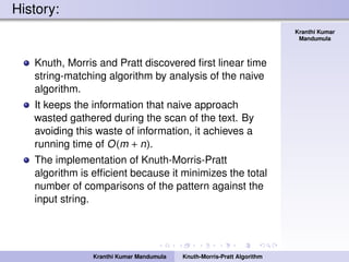
It preprocesses the pattern to find matches of
prefixes of the pattern with the pattern itself.
It is defined as the size of the largest prefix of
P[0..j − 1] that is also a suffix of P[1..j].
It also indicates how much of the last
comparison can be reused if it fails.
It enables avoiding backtracking on the string
‘S’.
Kranthi Kumar Mandumula Knuth-Morris-Pratt Algorithm

7. Knuth-Morris-Pratt
Algorithm
Kranthi Kumar
Mandumula
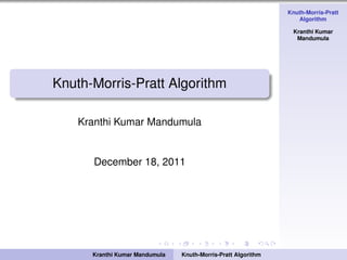
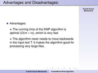
m ← length[p]
a[1] ← 0
k ← 0
for q ← 2 to m do
while k > 0 and p[k + 1] p[q] do
k ← a[k]
end while
if p[k + 1] = p[q] then
k ← k + 1
end if
a[q] ← k
end for
return
Here a =
Kranthi Kumar Mandumula Knuth-Morris-Pratt Algorithm

8. Knuth-Morris-Pratt
Algorithm
Kranthi Kumar
Mandumula
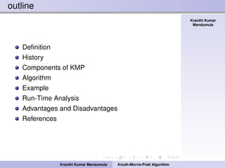
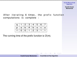
Computation of Prefix-function with example:
Let us consider an example of how to compute
for the pattern ‘p’.
Pattern a b a b a c a
I n i t i a l l y : m = length [ p]= 7
[1]= 0
k=0
where m, [1], and k are the length of the pattern,
prefix function and initial potential value
respectively.
Kranthi Kumar Mandumula Knuth-Morris-Pratt Algorithm

9. Knuth-Morris-Pratt
Algorithm
Kranthi Kumar
Mandumula
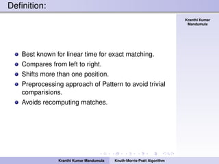
Step 1: q = 2 , k = 0
[2]= 0
q 1 2 3 4 5 6 7
p a b a b a c a
0 0
Step 2: q = 3 , k = 0
[3]= 1
q 1 2 3 4 5 6 7
p a b a b a c a
0 0 1
Kranthi Kumar Mandumula Knuth-Morris-Pratt Algorithm

10. Knuth-Morris-Pratt
Algorithm
Kranthi Kumar
Mandumula
Step 3: q = 4 , k = 1
[4]= 2
q 1 2 3 4 5 6 7
p a b a b a c a
0 0 1 2
Step 4: q = 5 , k = 2
[5]= 3
q 1 2 3 4 5 6 7
p a b a b a c a
0 0 1 2 3
Kranthi Kumar Mandumula Knuth-Morris-Pratt Algorithm

11. Knuth-Morris-Pratt
Algorithm
Kranthi Kumar
Mandumula
Step 5: q = 6 , k = 3
[6]= 1
q 1 2 3 4 5 6 7
p a b a b a c a
0 0 1 2 3 1
Step 6: q = 7 , k = 1
[7]= 1
q 1 2 3 4 5 6 7
p a b a b a c a
0 0 1 2 3 1 1
Kranthi Kumar Mandumula Knuth-Morris-Pratt Algorithm

12. Knuth-Morris-Pratt
Algorithm
Kranthi Kumar
Mandumula
After i t e r a t i n g 6 times , the p r e f i x function
computations i s complete :
q 1 2 3 4 5 6 7
p a b A b a c a
0 0 1 2 3 1 1
The running time of the prefix function is O(m).
Kranthi Kumar Mandumula Knuth-Morris-Pratt Algorithm

13. Knuth-Morris-Pratt
Algorithm
Kranthi Kumar
Mandumula
Algorithm
Step 1: I n i t i a l i z e the input variables :
n = Length of the Text .
m = Length of the Pattern .
= Prefix −function of pattern ( p ) .
q = Number of characters matched .
Step 2: Define the variable :
q=0 , the beginning of the match .
Step 3: Compare the f i r s t character of the pattern with f i r s t character of
t e x t .
I f match i s not found , s u b s t i t u t e the value of [ q ] to q .
I f match i s found , then increment the value of q by 1.
Step 4: Check whether a l l the pattern elements are matched with the t e x t
elements .
I f not , repeat the search process .
I f yes , p r i n t the number of s h i f t s taken by the pattern .
Step 5: look f o r the next match .
Kranthi Kumar Mandumula Knuth-Morris-Pratt Algorithm

14. Knuth-Morris-Pratt
Algorithm
Kranthi Kumar
Mandumula
n ← length[S]
m ← length[p]
a ← Compute Prefix function
q ← 0
for i ← 1 to n do
while q > 0 and p[q + 1] S[i] do
q ← a[q]
if p[q + 1] = S[i] then
q ← q + 1
end if
if q == m then
q ← a[q]
end if
end while
end for
Here a =
Kranthi Kumar Mandumula Knuth-Morris-Pratt Algorithm

15. Knuth-Morris-Pratt
Algorithm
Kranthi Kumar
Mandumula
Example of KMP algorithm:
Now let us consider an example so that the algorithm
can be clearly understood.
String b a c b a b a b a b a c a a b
Pattern a b a b a c a
Let us execute the KMP algorithm to find whether ‘p’
occurs in ‘S’.
Kranthi Kumar Mandumula Knuth-Morris-Pratt Algorithm

16. Knuth-Morris-Pratt
Algorithm
Kranthi Kumar
Mandumula
I n i t i a l l y : n = size of S = 15;
m = size of p=7
Step 1: i = 1 , q = 0
comparing p [ 1 ] with S[ 1 ]
String b a c b a b a b a b a c a a b
Pattern a b a b a c a
P[1] does not match with S[1]. ‘p’ will be shifted one position to the right.
Step 2: i = 2 , q = 0
comparing p [ 1 ] with S[ 2 ]
String b a c b a b a b a b a c a a b
Pattern a b a b a c a
Kranthi Kumar Mandumula Knuth-Morris-Pratt Algorithm

17. Knuth-Morris-Pratt
Algorithm
Kranthi Kumar
Mandumula
Step 3: i = 3 , q = 1
comparing p [ 2 ] with S[ 3 ] p [ 2 ] does not match with S[ 3 ]
String b a c b a b a b a b a c a a b
Pattern a b a b a c a
Backtracking on p , comparing p [ 1 ] and S[ 3 ]
Step 4: i = 4 , q = 0
comparing p [ 1 ] with S[ 4 ] p [ 1 ] does not match with S[ 4 ]
String b a c b a b a b a b a c a a b
Pattern a b a b a c a
Kranthi Kumar Mandumula Knuth-Morris-Pratt Algorithm

18. Knuth-Morris-Pratt
Algorithm
Kranthi Kumar
Mandumula
Step 5: i = 5 , q = 0
comparing p [ 1 ] with S[ 5 ]
String b a c b a b a b a b a c a a b
Pattern a b a b a c a
Step 6: i = 6 , q = 1
comparing p [ 2 ] with S[ 6 ] p [ 2 ] matches with S[ 6 ]
String b a c b a b a b a b a c a a b
Pattern a b a b a c a
Kranthi Kumar Mandumula Knuth-Morris-Pratt Algorithm

19. Knuth-Morris-Pratt
Algorithm
Kranthi Kumar
Mandumula
Step 7: i = 7 , q = 2
comparing p [ 3 ] with S[ 7 ] p [ 3 ] matches with S[ 7 ]
String b a c b a b a b a b a c a a b
Pattern a b a b a c a
Step 8: i = 8 , q = 3
comparing p [ 4 ] with S[ 8 ] p [ 4 ] matches with S[ 8 ]
String b a c b a b a b a b a c a a b
Pattern a b a b a c a
Kranthi Kumar Mandumula Knuth-Morris-Pratt Algorithm

20. Knuth-Morris-Pratt
Algorithm
Kranthi Kumar
Mandumula
Step 9: i = 9 , q = 4
comparing p [ 5 ] with S[ 9 ] p [ 5 ] matches with S[ 9 ]
String b a c b a b a b a b a c a a b
Pattern a b a b a c a
Step 10: i = 10 , q = 5
comparing p [ 6 ] with S[10] p [ 6 ] doesn ’ t matches with S[10]
String b a c b a b a b a b a c a a b
Pattern a b a b a c a
Backtracking on p , comparing p [ 4 ] with S[10] because a f t e r mismatch q = [ 5 ] = 3
Kranthi Kumar Mandumula Knuth-Morris-Pratt Algorithm

21. Knuth-Morris-Pratt
Algorithm
Kranthi Kumar
Mandumula
Step 11: i = 11 , q = 4
comparing p [ 5 ] with S[11]
String b a c b a b a b a b a c a a b
Pattern a b a b a c a
Step 12: i = 12 , q = 5
comparing p [ 6 ] with S[12] p [ 6 ] matches with S[12]
String b a c b a b a b a b a c a a b
Pattern a b a b a c a
Kranthi Kumar Mandumula Knuth-Morris-Pratt Algorithm

22. Knuth-Morris-Pratt
Algorithm
Kranthi Kumar
Mandumula
Step 13: i = 13 , q = 6
comparing p [ 7 ] with S[13] p [ 7 ] matches with S[13]
String b a c b a b a b a b a c a a b
Pattern a b a b a c a
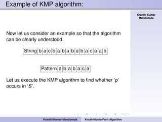
pattern ‘p’ has been found to completely occur in
string ‘S’. The total number of shifts that took place for
the match to be found are: i − m = 13-7 = 6 shifts.
Kranthi Kumar Mandumula Knuth-Morris-Pratt Algorithm

23. Knuth-Morris-Pratt
Algorithm
Kranthi Kumar
Mandumula
Run-Time analysis:
O(m) - It is to compute the prefix function values.
O(n) - It is to compare the pattern to the text.
Total of O(n + m) run time.
Kranthi Kumar Mandumula Knuth-Morris-Pratt Algorithm

24. Knuth-Morris-Pratt
Algorithm
Kranthi Kumar
Mandumula
Advantages and Disadvantages:
Advantages:
The running time of the KMP algorithm is
optimal (O(m + n)), which is very fast.
The algorithm never needs to move backwards
in the input text T. It makes the algorithm good for
processing very large files.
Kranthi Kumar Mandumula Knuth-Morris-Pratt Algorithm

25. Knuth-Morris-Pratt
Algorithm
Kranthi Kumar
Mandumula
Advantages and Disadvantages:
Disadvantages:
Doesn’t work so well as the size of the
alphabets increases. By which more chances of
mismatch occurs.
Kranthi Kumar Mandumula Knuth-Morris-Pratt Algorithm

26. Knuth-Morris-Pratt
Algorithm
Kranthi Kumar
Mandumula
Graham A.Stephen, “String Searching Algorithms”,
year = 1994.
Donald Knuth, James H. Morris, Jr, Vaughan Pratt,
“Fast pattern matching in strings”, year = 1977.
Thomas H.Cormen; Charles E.Leiserson.,
Introduction to algorithms second edition , “The
Knuth-Morris-Pratt Algorithm”, year = 2001.
Kranthi Kumar Mandumula Knuth-Morris-Pratt Algorithm