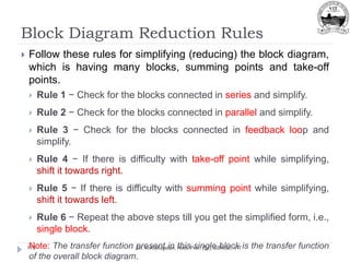
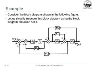
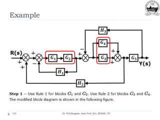
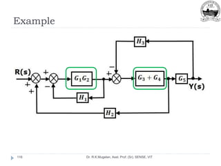
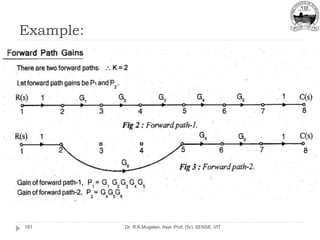
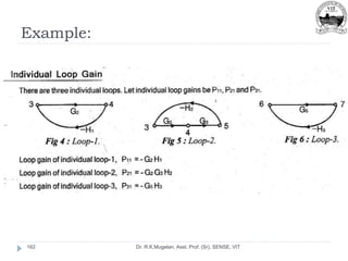
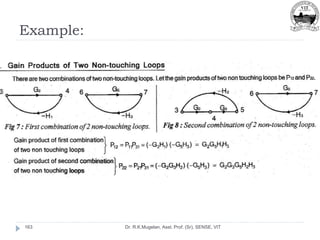
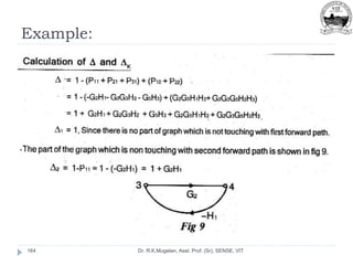
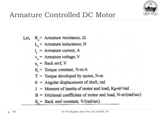
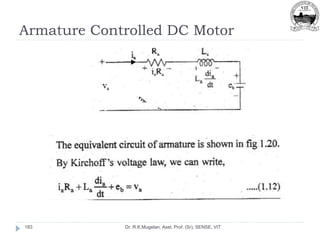
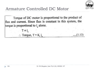
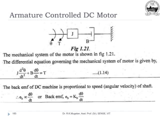
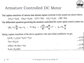
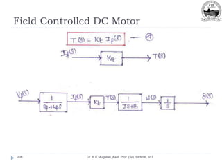
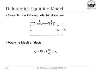
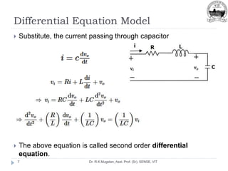
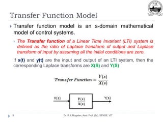
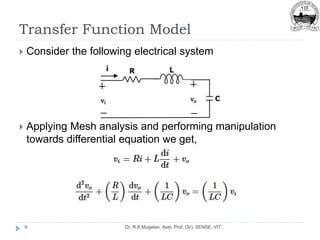
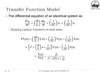
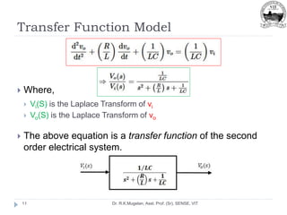
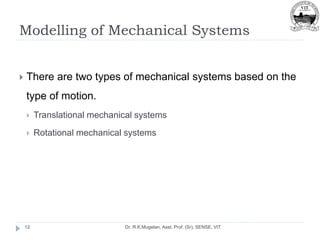
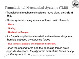
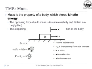
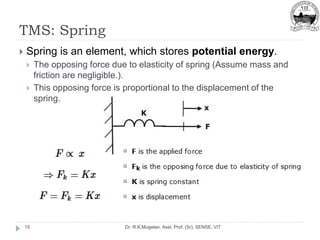
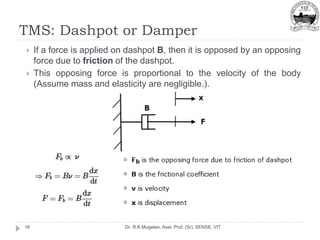
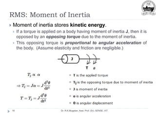
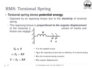
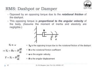
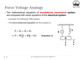
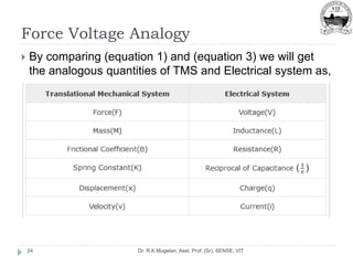
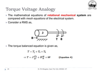
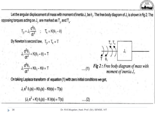
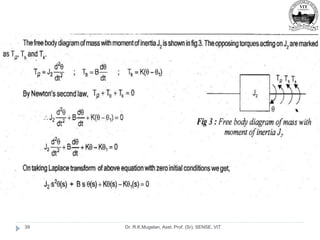
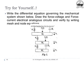
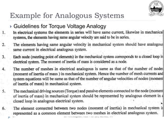
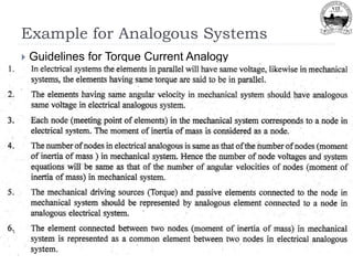
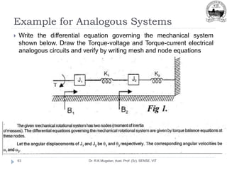
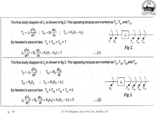
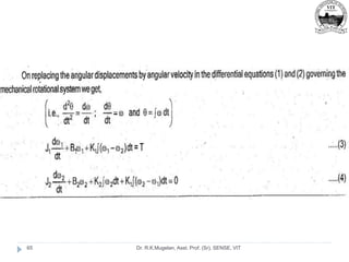
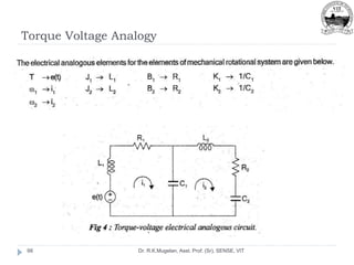
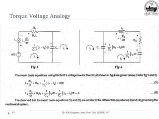
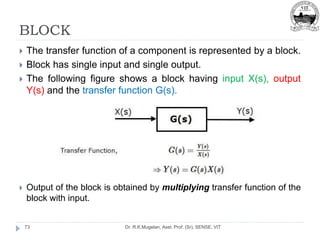
This document outlines Module 2 of a course on mathematical modeling of physical systems. It discusses different modeling approaches including differential equation, transfer function, and state-space models. It covers modeling of electrical, translational mechanical, and rotational mechanical systems. Translational systems are modeled using mass, spring, and damper elements, while rotational systems use moment of inertia, torsional spring, and damper. Analogies between electrical and mechanical systems allow representing one in terms of the other. The force-voltage and torque-voltage analogies map mechanical forces and torques to electrical voltages, while force-current and torque-current analogies map them to currents. Examples are provided to derive the differential equations and transfer functions of systems.


![Solution
Dr. R.K.Mugelan, Asst. Prof. (Sr), SENSE, VIT
59
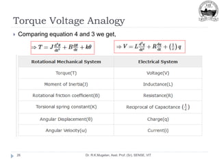
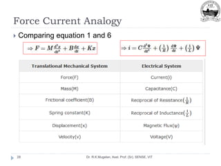
On comparing equations (3) and (4) [Mechanical System]
with expressions (5), (6)[Force Voltage Analogy] and
expressions (6), (7) [Force Current Analogy]](https://image.slidesharecdn.com/module-2-220916105551-78737c58/85/Module-2-pptx-59-320.jpg)
![Solution
Dr. R.K.Mugelan, Asst. Prof. (Sr), SENSE, VIT
70
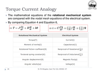
On comparing equations (3) and (4) [Mechanical System] with
expressions (5), (6)[Torque Voltage Analogy] and expressions (6), (7)
[Torque Current Analogy]](https://image.slidesharecdn.com/module-2-220916105551-78737c58/85/Module-2-pptx-70-320.jpg)
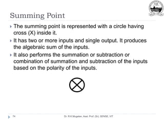
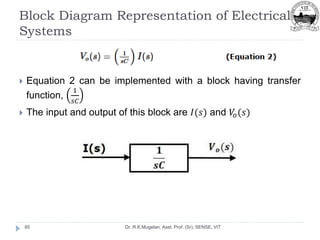
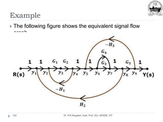
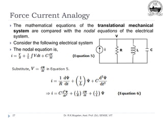
![Summing Point
Dr. R.K.Mugelan, Asst. Prof. (Sr), SENSE, VIT
75
The following figure shows the summing point with two inputs
(A, B) and one output (Y).
Here, the inputs A and B have a positive sign.
So, the summing point produces the output, Y as sum of A
and B. [Y=A+B]](https://image.slidesharecdn.com/module-2-220916105551-78737c58/85/Module-2-pptx-75-320.jpg)
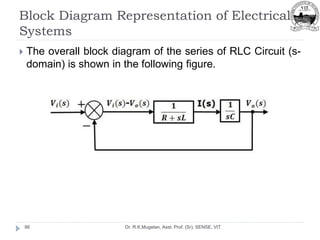
![Summing Point
Dr. R.K.Mugelan, Asst. Prof. (Sr), SENSE, VIT
76
The following figure shows the summing point with two inputs
(A, B) and one output (Y).
Here, the inputs A and B are having opposite signs, i.e., A is
having positive sign and B is having negative sign.
So, the summing point produces the output Y as the
difference of A and B. [Y=A+(-B)=A-B]](https://image.slidesharecdn.com/module-2-220916105551-78737c58/85/Module-2-pptx-76-320.jpg)