The document outlines the implementation of the reciprocity theorem, which states that the current from a voltage source at one point is equal to the current at the other point when positions are interchanged. It includes details on the objectives, theory, apparatus, procedure, calculations, and results of an experiment conducted to demonstrate the theorem using a circuit with resistors and a breadboard setup. The results showed a 4% error in the current measurements, confirming the theorem's validity under specified conditions.

1. IMPLIMENTATION OF RECIPROCITY THEOREM

2. CONTENTS OF THE
PRESENTATION
 Objectives
 introduction
 Theory
 Apparatus
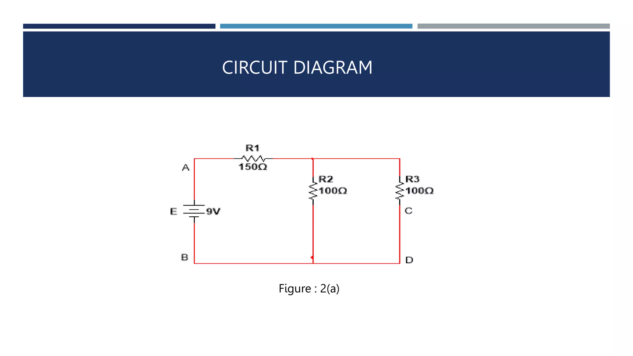
 Circuit Diagram
 Procedure
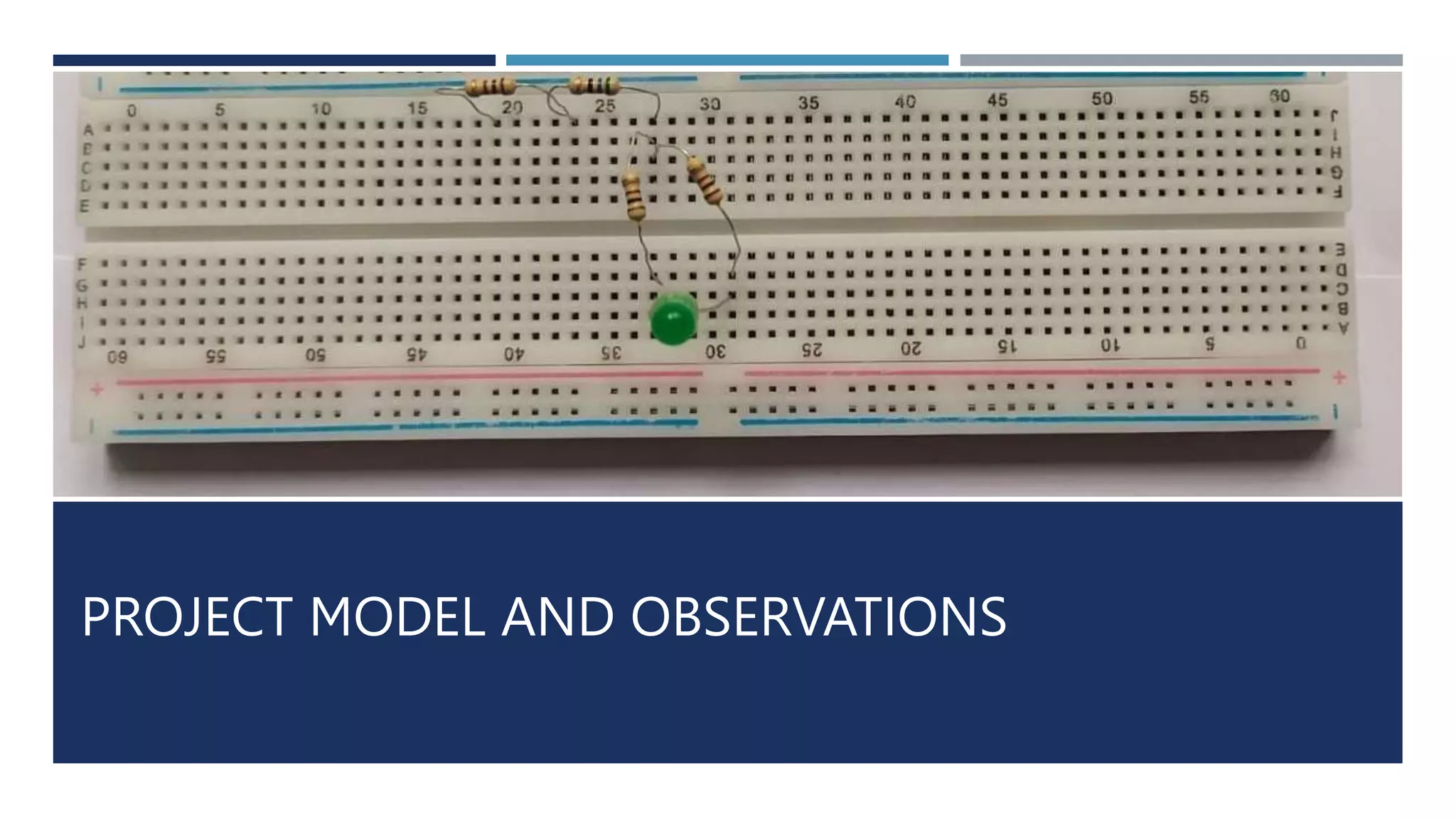
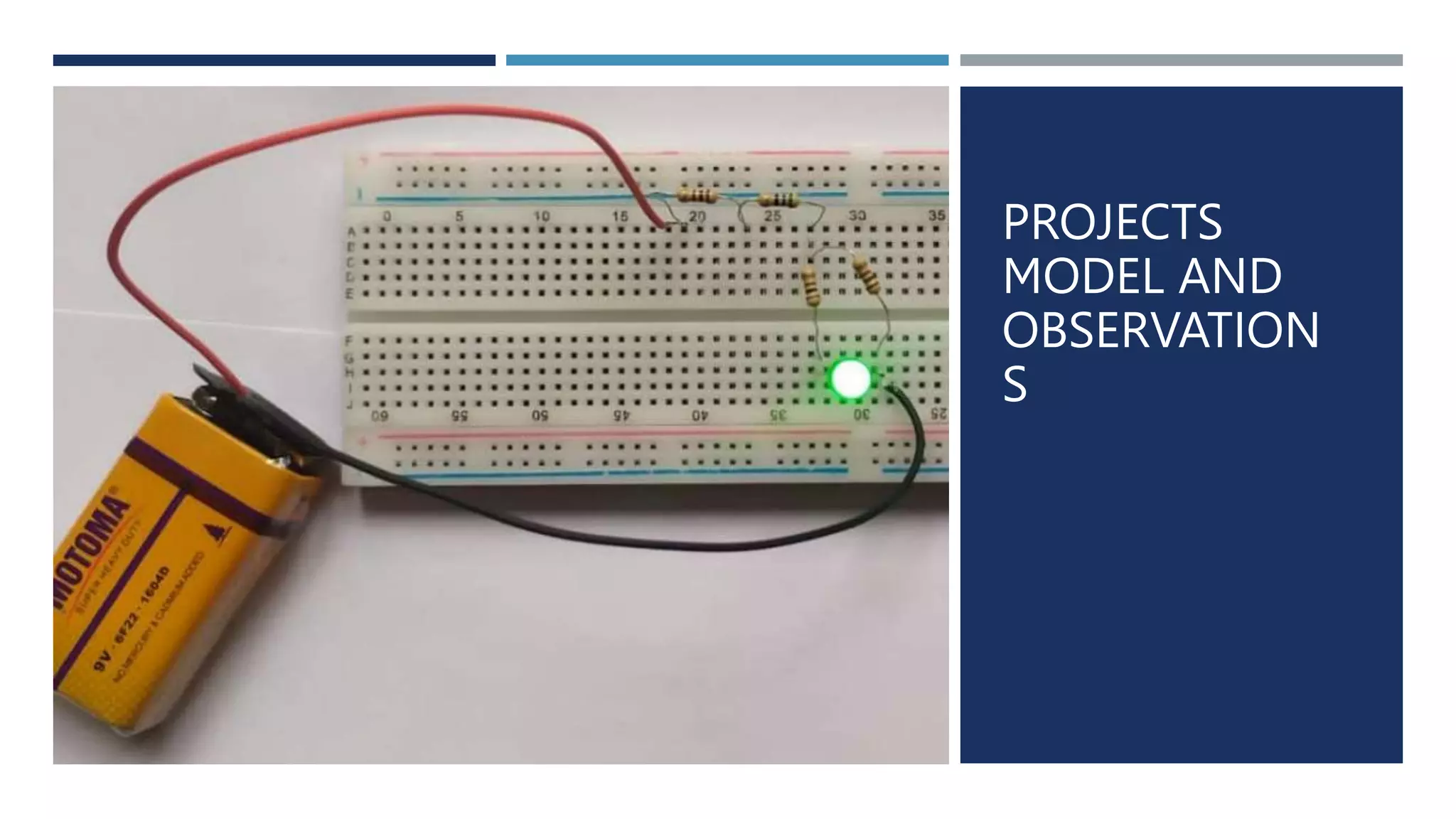
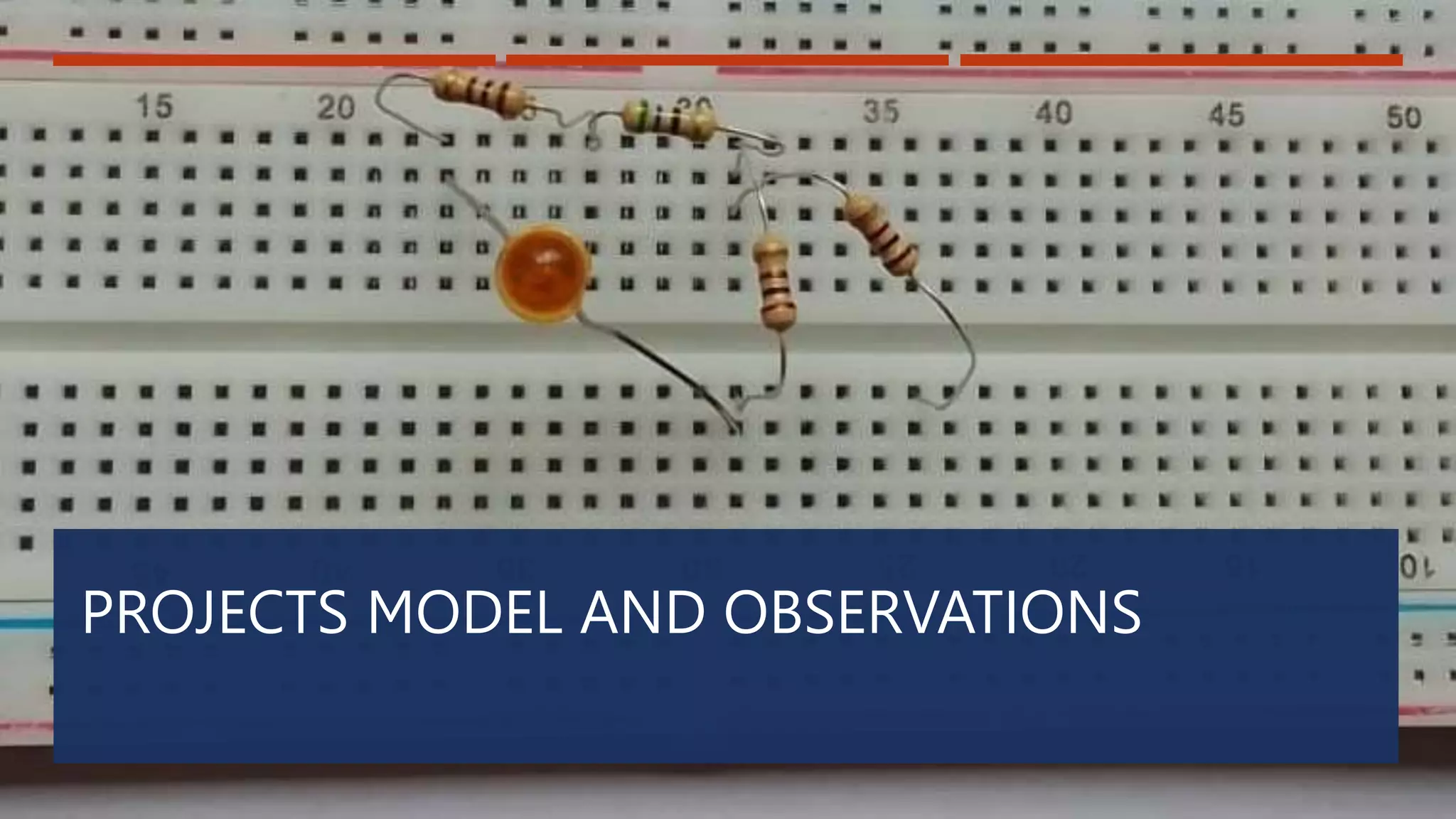
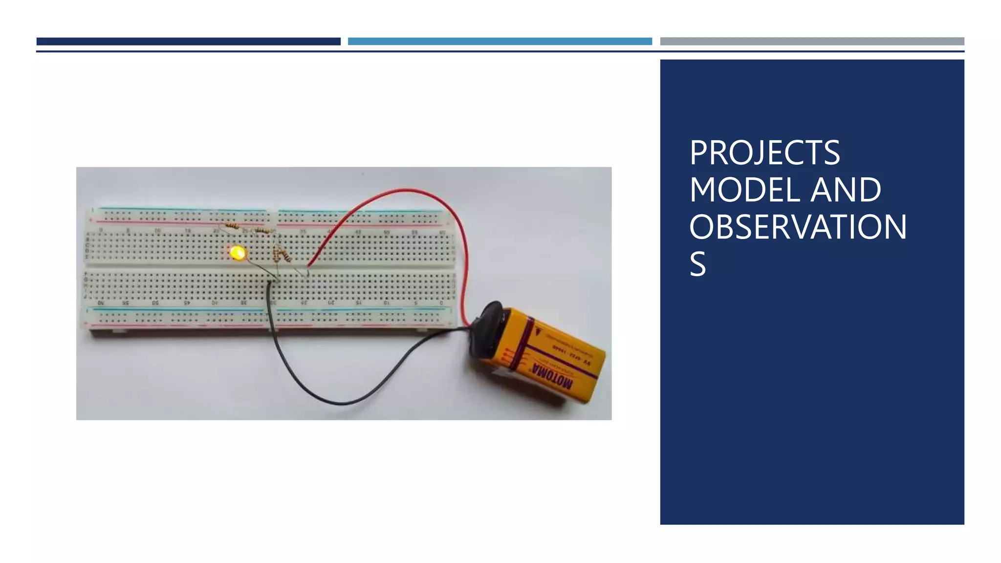
 project model and
observations
 Calculation
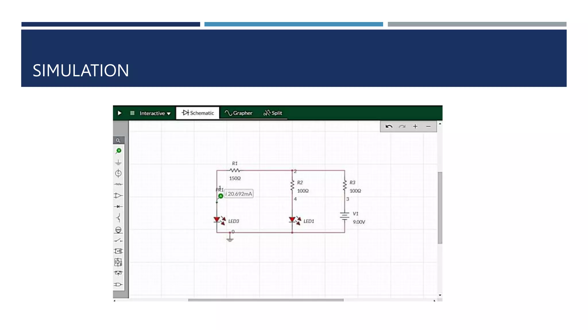
 simulation
 Result

3. OBJECTIVES AND OUTCOMES
 Understanding what Reciprocity Theorem
 Understanding how Reciprocity Theorem work
 Implementation of Reciprocity Theorem in a breadboard and simulation
 Proving Reciprocity Theorem

4. INTRODUCTION
The principle of reciprocity in acoustic as well as electromagnetic (EM)
systems was first enunciated by Lord Rayleigh. Soon afterward, H. A. Lorentz and
J. R. Carson extended the concept and provided sound physical and mathematical arguments that
underlie the rigorous proof of the reciprocity theorem. Over the years, the theorem has been
embellished and extended to cover a broader range of possibilities, and to apply with fewer
constraints The basic concept and its proof based on Maxwell’s macroscopic equations
are discussed in standard textbooks on electromagnetism. For a recent review of
reciprocity in optics, the reader is referred to the comprehensive article by Potton.

5. THEORY
 The reciprocity theorem states that the current at one point in a circuit due to a voltage at a second
point is the same as the current at the second point due to the same voltage at the first.
 The limitation of this theorem is that it is applicable only to single-source networks and not in the multi-
source network.
 The network where reciprocity theorem is applied should be linear and consist of resistors, inductors,
capacitors and coupled circuits.
 The circuit should not have any time-varying elements.

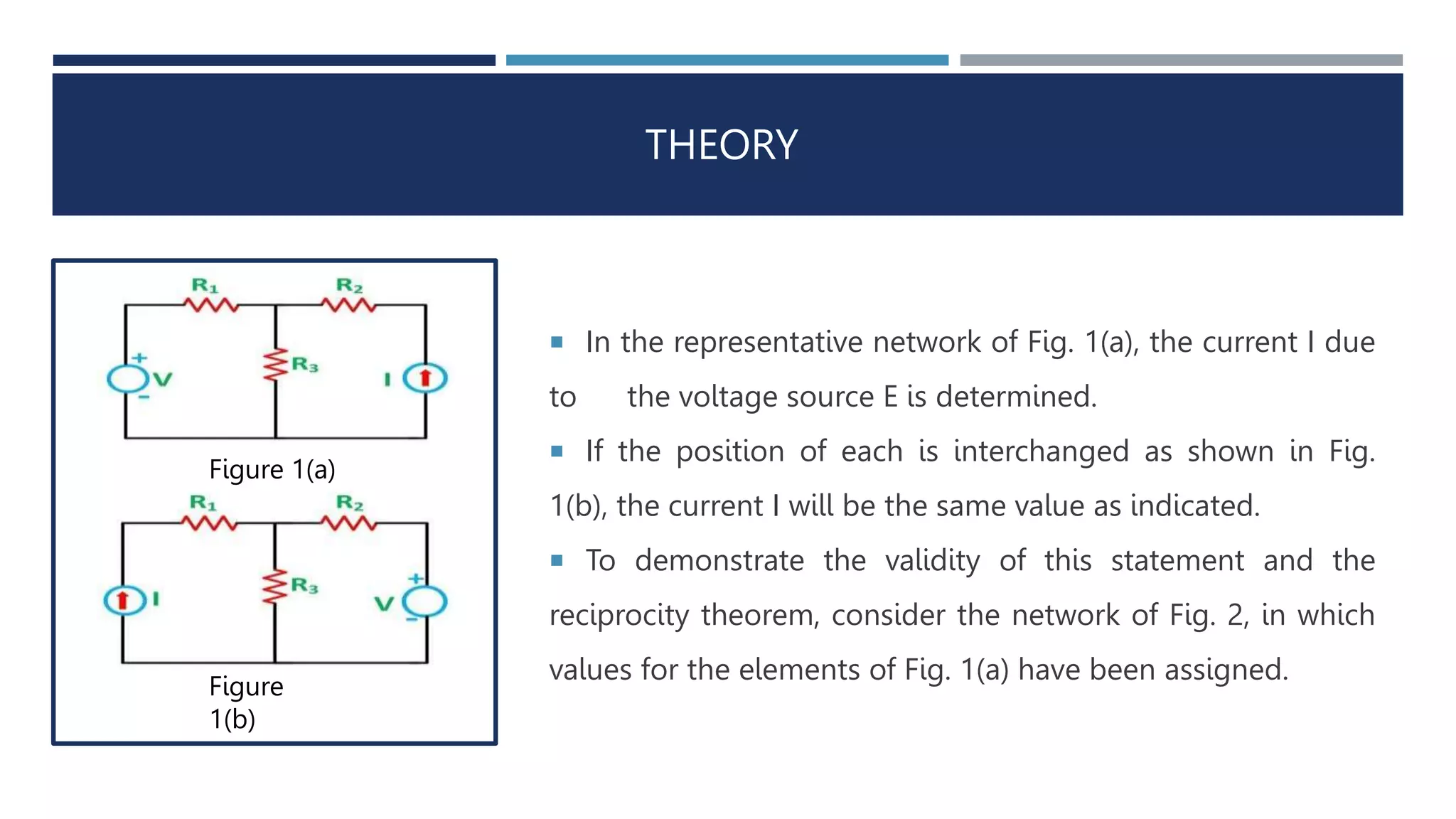
6.  In the representative network of Fig. 1(a), the current I due
to the voltage source E is determined.
 If the position of each is interchanged as shown in Fig.
1(b), the current I will be the same value as indicated.
 To demonstrate the validity of this statement and the
reciprocity theorem, consider the network of Fig. 2, in which
values for the elements of Fig. 1(a) have been assigned.
THEORY
Figure 1(a)
Figure
1(b)

7. APPARATUS
 Resistor ( 150Ω, 100Ω , 100Ω )
 Source ( 9 V )
 Breadboard
 LED Light ( 0.02 A )
 Connecting Wire

8. CIRCUIT DIAGRAM
Figure : 2(a)

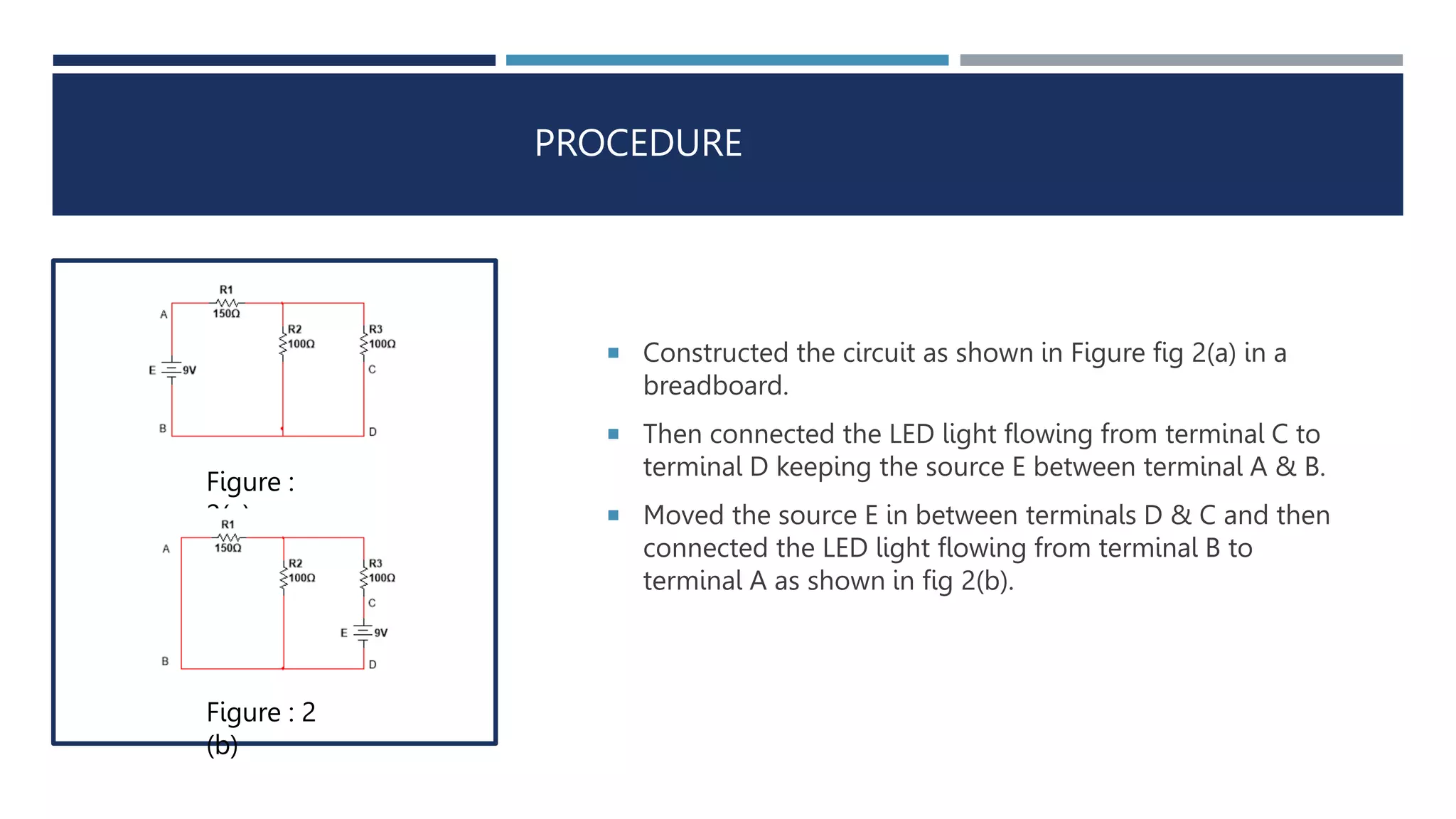
9. PROCEDURE
 Constructed the circuit as shown in Figure fig 2(a) in a
breadboard.
 Then connected the LED light flowing from terminal C to
terminal D keeping the source E between terminal A & B.
 Moved the source E in between terminals D & C and then
connected the LED light flowing from terminal B to
terminal A as shown in fig 2(b).
Figure :
2(a)
Figure : 2
(b)

10. PROJECT MODEL AND OBSERVATIONS

11. PROJECTS
MODEL AND
OBSERVATION
S

12. PROJECTS MODEL AND OBSERVATIONS

13. PROJECTS
MODEL AND
OBSERVATION
S

14. SIMULATION

15. SIMULATION

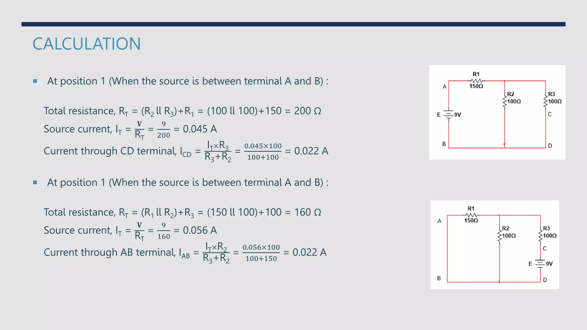
16. CALCULATION
 At position 1 (When the source is between terminal A and B) :
Total resistance, RT = (R2 ll R3)+R1 = (100 ll 100)+150 = 200 Ω
Source current, IT =
𝐕
RT
=
9
200
= 0.045 A
Current through CD terminal, ICD =
IT×R3
R3+R2
=
0.045×100
100+100
= 0.022 A
 At position 1 (When the source is between terminal A and B) :
Total resistance, RT = (R1 ll R2)+R3 = (150 ll 100)+100 = 160 Ω
Source current, IT =
𝐕
RT
=
9
160
= 0.056 A
Current through AB terminal, IAB =
IT×R2
R3+R2
=
0.056×100
100+150
= 0.022 A

17. RESULTS
 Error in currents value
=
0.022−0.021
0.021
× 100
= 4% 𝑒𝑟𝑟𝑜𝑟

18. Thank You