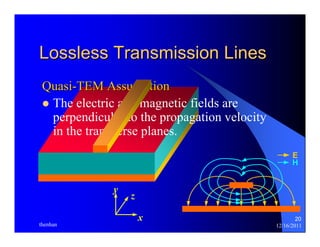
The document provides information on microwave engineering and transmission lines. It discusses topics such as the frequency range of microwave engineering (1 GHz and above), transmission line theory, characteristic impedance, propagation velocity, lossless transmission lines, and formulas for calculating the characteristic impedance of different transmission line structures including coaxial cable, striplines, and dual striplines.

1. MICROWAVE ENGINEERING
LECTURE NOTE
1
thenhan 12/16/2011

2. 2
PHẠẠM VI CỦỦA LĨĨNH VỰỰC SIÊU
CAO TẦẦN
z TẦN SỐ THÔNG THƯỜNG TỪ 1GHz
TRỞ LÊN
BẢNG PHÂN ĐỊNH TẦN SỐ
thenhan 12/16/2011

3. 3
thenhan 12/16/2011

4. 4
thenhan 12/16/2011

5. 5
thenhan 12/16/2011

6. 6
ĐĐƯƯỜỜNG DÂY TRUYỀỀN SÓNG
. ĐIỆN ÁP VÀ DÒNG ĐIỆN PHỤ THUỘC CẢ
KHÔNG GIAN Ở VỊ TRÍ z VÀ THỜI GIAN TẠI
THỜI ĐIỂM t,
thenhan 12/16/2011

7. Module 2: Transmission Lines
Topic 1: Theory
7
OGI EE564
Howard Heck
thenhan 12/16/2011

8. 8
Where Are We? 1. Introduction
2. Transmission Line Basics
1. Transmission Line Theory
2. Basic I/O Circuits
3. Reflections
4. Parasitic Discontinuities
5. Modeling, Simulation, & Spice
6. Measurement: Basic Equipment
7. Measurement: Time Domain Reflectometry
3. Analysis Tools
4. Metrics & Methodology
5. Advanced Transmission Lines
thenhan 12/16/2011

9. 9
CzoPnrotpeangattsion Velocity
z Characteristic Impedance
z Visualizing Transmission Line Behavior
z General Circuit Model
z Frequency Dependence
z Lossless Transmission Lines
z Homogeneous and Non-homogeneous Lines
z Impedance Formulae for Transmission Line
Structures
z Summary
z References
thenhan 12/16/2011

10. y
I+ d I dz
dz
V+ d V dz
z
x
[2.1.1]
[2.1.2]
I
V
C V
I
∂
∂
= −
Ldz
Cdz
dz
dz
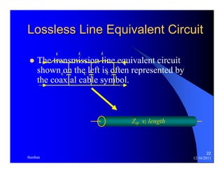
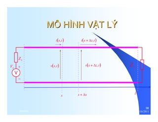
V, I
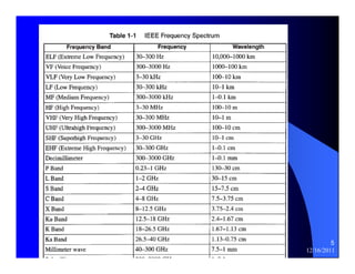
the Telegraphist’s Equations [2.1.3a]
[2.1.3b]
10
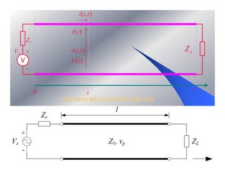
Wave propagates in z Propagation direction
Velocity
z Physical example:
9 Circuit: L = [nH/cm]
C = [pF/cm]
V
dz ( Ldz )
I
z
∂
t
∂
∂
9 Total voltage change across = −
∂
Ldz (use Δ V L d I ):
= − dt
9 Total current change across
ΔI = −C dV
Cdz (use d t ):
I
∂
dz ( Cdz )
V
z
t
∂
∂
∂
= −
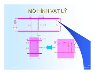
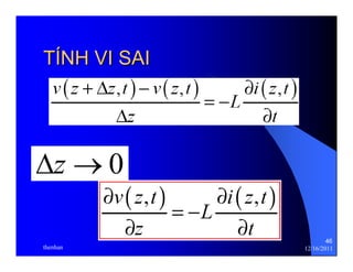
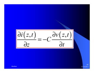
9 Simplify [2.1.1] & [2.1.2] to get
t
∂
L I
∂
t
z
∂
V
∂
z
∂
∂
= −
thenhan 12/16/2011

11. 2 2
C V
I
∂
∂
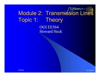
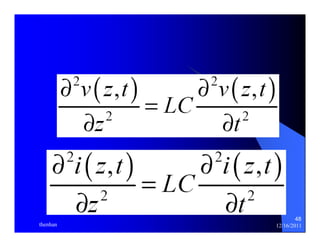
9 Differentiate [2.1.3a] by t: 2 [2.1.4]
t
z t
∂
= −
∂ ∂
∂ 2
L I
2
V
∂
9 Differentiate [2.1.3b] by z: [2.1.5]
2
t z
z
∂ ∂
= −
∂
2
2 2
1
V
LC V
V
∂
∂
∂
9 Equate [2.1.4] & [2.1.5]: [2.1.6] 2
[2.1.7]
[2.1.8]
11
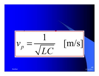
Propagation Velocity (2)
∂
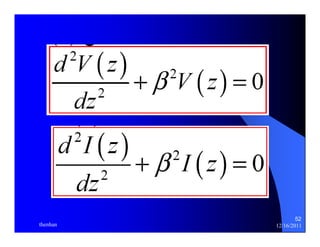
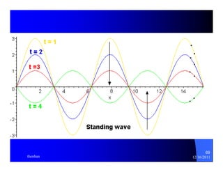
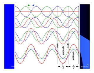
9 Equation [2.1.6] is a form of the wave equation. The solution to
[2.1.6] contains forward and backward traveling wave
components, which travel with a phase velocity.
9 Phase velocity definition: v
2
z
=
≡ 1
LC
9 Equation in terms of current:
t
∂
I
2
2
=
2 2
t
∂
ν
2 1
LC I
=
2 2
2
I
2
t
t
z
∂
∂
∂
∂
=
∂
∂
ν
An alternate treatment of propagation velocity is contained in the appendix.
thenhan 12/16/2011

12. dz = segment length
C = capacitance per segment
L = inductance per segment
12
Z1 Z2 Z3
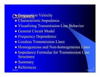
Characteristic Impedance
b c
Ldz
(Lossless)
V1 V2 V3 Cdx
to ∞
Ldz
Cdz
Ldz
Cdz
d e f
dz dz
a
dz
z The input impedance (Z1) is the impedance
of the first inductor (Ldz) in series with the
parallel combination of the impedance of
the capacitor (Cdz) and Z2.
[2.1.9]
( )
Z j Cdz
Z j Ldz Z j ω
Cdz
ω
= ω
+
1/
2
1/
2
1 +
( 1/ ) ( 1/ ) (1/ ) 0 1 2 2 2 Z Z + jωlC − jωlL Z + jωlC − Z jωlC =
thenhan 12/16/2011

13. 13
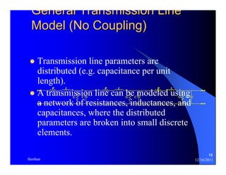
Characteristic Impedance
(Lossless)
z Assuming a uniform line, the input
impedance should be the same when
looking into node pairs a-d, b-e, c-f, and so
fo( rth1./ So, Z) 2 = Z(1= 1Z/0. ) (1/ ) 0 0 0 0 0 Z Z + jωCdz − jωlLdz Z + jωCdz − Z jωCdz = [2.1.10]
ω
Z j LZ dz j Ldz
j Cdz
Z
2
0
2 0
0 0
+ − − − 0
= = − 0
− j Cdz
ω
j LZ dz Ldz
Cdz
Z Z
j Cdz
ω
ω
ω ω
ω
ω
0
Z 2
− jωLZ L 0 0
dz − =
0 [2.1.11]
C
9 Allow dz to become very small, causing the frequency
dependent term to drop out:
Z L [2.1.12]
2 0
0 − =
C
9 Solve for Z0:
Z = L 0
C
[2.1.13]
thenhan 12/16/2011

14. 14
Visualizing Transmission Line
h
Behavior
f
z Water flow
– Potential = Wave
height [m]
– Flow = Flow rate
[liter/sec]
I
+++++++
- - - - - - -
I
V
9 Transmission Line
¾ Potential = Voltage [V]
¾ Flow = Current [A] =
[C/sec]
9 Just as the wave front of the water flows in the pipe, the
voltage propagates in the transmission line. The same
holds true for current.
¾ Voltage and current propagate as waves in the transmission line.
thenhan 12/16/2011

15. 15
Visualizing Transmission Line
Behavior #2
z Extending the analogy
– The diameter of the pipe relates the flow rate
and height of the water. This is analogous to
electrical impedance.
– Ohm’s law and the characteristic impedance
define the relationship between current and
potential in the transmission line.
z Effects of impedance discontinuities
– What happens when the water encounters a
ledge or a barrier?
– What happens to the current and voltage
waves when the impedance of the
transmission line changes?
thenhan 12/16/2011

16. 16
General Transmission Line
Model (No Coupling)
z Transmission line parameters are
distributed (e.g. capacitance per unit
length).
R L
R L
R L
z A G C
transmission line can G be C
modeled G C
using
a network of resistances, inductances, and
capacitances, where the distributed
parameters are broken into small discrete
elements.
thenhan 12/16/2011

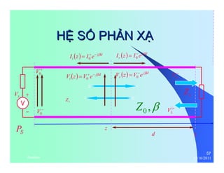
17. ω
ω [2.1.14]
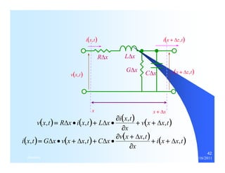
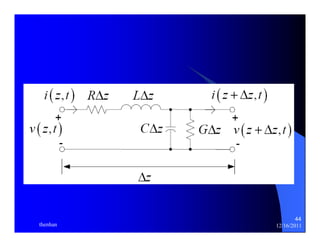
Propagation Constant γ = (R + jωL)(G + jωC) =α + jβ [2.1.15]
α = attenuation constant = rate of exponential attenuation
β = phase constant = amount of phase shift per unit length
ν = Phase Velocity p [2.1.16]
In general, α and β are frequency dependent.
17
General Transmission Line
Model #2
Symb Units
ol
Parameters Parameter
Conductor R Ω•cm-1
Resistance
Self Inductance L nH•cm-1
Total Capacitance C pF•cm-1
Ω-1•cm -
1 Dielectric G
Conductance
Characteristic Impedance Z R j L
+
+
0 G j C =
ω
β
thenhan 12/16/2011

18. 18
Frequency Dependence
From [2.1.14] and [2.1.15] note that:
z Z0 and γ depend on the frequency content
of the signal.
z Frequency dependence causes attenuation
and edge rate degradation.
Attenuation
Output signal from lossy
transmission line
Output signal from
lossless transmission line
Edge rate degradation
Signal at driven end of
transmission line
thenhan 12/16/2011

19. 19
FrzeRqaunede nGncarye sDomeeptiemnesd neegnlicgiebl e#, 2
particularly at low frequencies
– Simplifies to the lossless case: no attenuation
& no dispersion
z In modules 2 and 3, we will concentrate on
lossless transmission lines.
z Modules 5 and 6 will deal with lossy lines.
thenhan 12/16/2011

20. H E
20
Lossless Transmission Lines
Quasi-TEM Assumption
z The electric and magnetic fields are
perpendicular to the propagation velocity
in the transverse planes.
x
y z
thenhan 12/16/2011

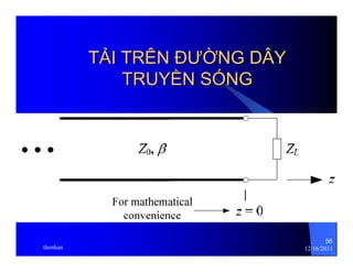
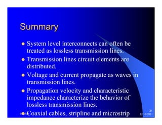
21. 21
z Lossless transmission lines are characterized
by the following two parameters:
Lossless Line Parameters
Z = L 0
C
v
= 1
LC
Characteristic Impedance
Propagation Velocity
z Lossless line characteristics are frequency
independent.
z As noted before, Z0 defines the relationship
between voltage and current for the traveling
waves. The units are ohms [Ω].
z υ defines the propagation velocity of the
waves. The units are cm/ns.
thenhan 12/16/2011
S ti th ti dl
[2.1.17]
[2.1.18]

22. 22
Lossless Line Equivalent Circuit
L
L
L
z The transmission line equivalent circuit
shown C
on the C
left is C
often represented by
the coaxial cable symbol.
Z0Z, 0ν, ,v l,e lnegntghth
thenhan 12/16/2011

23. [2.1.19]
23
Homogeneous Media
z A homogeneous dielectric medium is
uniform in all directions.
– All field v
= 1 lines = are 1 = 0 = contained 30
within the
dielectric.
LC
c cm /
ns
εμ ε μ ε
r r r
0 ε ε ε r = Dielectric Permittivity
εNote: only r
r
εz For a ε 0 = 8.854 x transmission 10− 14 F
line in a Permittivity of free homogeneous
space
medium, μ the cm
8 0 =1.257 x 10− H
propagation velocity depends
only on material cm
properties:
Magnetic Permeability
0 μ ≅ μ Permeability of free space
εr
is the relative permittivity or dielectric constant.
is required to
calculate νν.
thenhan 12/16/2011

24. 24
Non-Homogeneous Media
z A non-homogenous medium contains
multiple materials with different dielectric
constants.
z For a non-homogeneous medium, field
lines cut v
= 1 ≠ 1
across LC
the εμ
boundaries between
dielectric materials.
z In this case the propagation velocity
depends on the dielectric constants and the
proportions of the materials. Equation
[2.1.19] does not hold:
9 In practice, an effective dielectric constant, εr,eff is
often used, which represents an average dielectric
constant.
thenhan 12/16/2011

25. 25
Some Typical Transmission
Line Structures
And useful formulas for Z0
thenhan 12/16/2011

26. 26
r
R
εr
Trởở kháng cáp đđồồng trụục
εr = 2
εr = 2.5
εr = 3
2 3 4 5 6 7 8 9 10
R/r
140
120
100
80
60
40
20
⎞
Z = 1
ln ⎛
R
0 ε
2πε
⎞
⎛
R
⎞
μ
L = ln ⎛
R
thenhan 12/16/2011
Z0 [ Ω]
εr
= 1
εrr= 4 ε = 3.5
, lZe0n, gυth, vle, n0gZth
⎟⎠
⎜⎝
r
2
μ
π
[2.1.20]
⎟⎠
⎜⎝
=
r
C
ln
[2.1.21]
⎟⎠
⎜⎝
r
2π
[2.1.22]

27. ⎞
h
4
60 ln 2
( )⎟ ⎟ ⎟
⎠
w
0.35
0.25
27
Centered Stripline Impedance
⎛
⎜ ⎜ ⎜
0 ε π
r 0.67 0.8
⎝
w +
t
=
Z
w
t
h1
h2
εr
Source: Motorola
application note
AN1051.
Valid for w
h −t
2
<
h <
2
t
60 Z0 [Ω]
55
50
45
40
35
30
25
20
15
h2
0.003 0.005 0.007 0.009 0.011 0.013 0.015
thenhan 12/16/2011
w [in]
10
0.070
0.060
0.050
0.040
0.030
0.025
0.020
t = 0.0007”
εr = 4.0

28. [2.1.24]
[2.1.25]
[2.1.26]
[2.1.27]
28
Dual Stripline Impedance
w
h1
t
h2
Z YZ
⎞
⎛
Y h
60 ln 8 1
ε π
⎞
⎛
Z h h
60 ln 8 1 2
ε π
⎤
1
h h t h t
ln ⎡
1.9 2
+
⎤
⎡
⎞
⎛
110
100
90
80
70
60
50
40
30
20
thenhan 12/16/2011
εr
w
t
h1
Y +
Z
= 2
0
( )⎟ ⎟ ⎟
⎠
⎜ ⎜ ⎜
⎝
+
=
w
w t
r 0.67 0.8
( )
( )⎟ ⎟ ⎟
⎠
⎜ ⎜ ⎜
⎝
+
+
=
w
w t
r 0.67 0.8
( ) ( )
⎥⎦
⎢⎣
+
⎥⎦
⎢⎣
⎟ ⎟⎠
⎜ ⎜⎝
+ +
−
=
w t
h
Z
r 0.8
4
80 1
1 2 1
0 ε
1 1. 0.5h ≤ w ≤ h
Source: Motorola
application note
AN1051.
OR
0.003 0.005 0.007 0.009 0.011 0.013 0.015
w [in]
10
Z0 [ Ω]
0.020”
0.018”
0.015”
0.012”
0.010”
0.008”
0.005”
2h1 + h2 + 2t = 0.062”
t = 0.0007”
εr = 4.0
h1

29. 29
Surface Microstrip Impedance
w
t
h
⎞
Z = 1
⎛
h
0 ε
⎞
Z h
ln ⎛
5.98
87
160
140
120
100
80
60
40
h
thenhan 12/16/2011
ε0
εr
[ ] Ω ⎟⎠
⎜⎝
d
eff
ln 4
2
μ
π
d = 0.536w+ 0.67t
( ) 0 ε = 0.475ε + 0.67 ε eff r
[ ] Ω ⎟⎠
⎜⎝
+ +
=
w t
r 1.41
0.8
0 ε
0.003 0.005 0.007 0.009 0.011 0.013 0.015
w [in]
20
Z0 [Ω]
0.025”
0.020”
0.015”
0.012”
0.009”
0.006”
0.004”
t = 0.0007”
εr
= 4.0
[2.1.28]
[2.1.29]
[2.1.30]
[2.1.31]

30. [2.1.32]
[2.1.33]
[2.1.34]
[2.1.35]
30
Embedded Microstrip
t
h1
ε0
εr
w
h2
⎞
⎟⎠
Z K ln ⎛
5.98
h
⎜⎝
1
w t
0 ε
where 60 ≤ K ≤ 65
r 0.8
+ +
=
0.805 2
⎞
⎟⎠
Z h
ln 5.98
87 ⎛
1
⎜⎝
0 ε
[1 1.55h2 h1 ]
r r eε ′ =ε − −
=1.017 0.475 + 0.67 r ε
w t
r 0.8
′ + +
=
1.41
τ
Or
140
120
100
80
60
40
20
0
h1
0.015”
0.012”
0.010”
0.008”
0.006”
0.005”
0.003”
h2 - h1 = 0.002“
t= 0.0007”
εr
= 4.0
0.003 0.005 0.007 0.009 0.011 0.013 0.015
w [in]
Z0 [Ω]
thenhan 12/16/2011

31. 31
Summary
z System level interconnects can often be
treated as lossless transmission lines.
z Transmission lines circuit elements are
distributed.
z Voltage and current propagate as waves in
transmission lines.
z Propagation velocity and characteristic
impedance characterize the behavior of
lossless transmission lines.
z Coaxial cables, stripline and microstrip
thenhan 12/16/2011

32. 32
References
z S. Hall, G. Hall, and J. McCall, High Speed
Digital System Design, John Wiley & Sons, Inc.
(Wiley Interscience), 2000, 1st edition.
z H. Johnson and M. Graham, High-Speed Signal
Propagation: Advanced Black Magic, Prentice
Hall, 2003, 1st edition, ISBN 0-13-084408-X.
z W. Dally and J. Poulton, Digital Systems
Engineering, Cambridge University Press, 1998.
z R.E. Matick, Transmission Lines for Digital and
Communication Networks, IEEE Press, 1995.
z R. Poon, Computer Circuits Electrical Design,
Prentice Hall 1st edition 1995
thenhan 12/16/2011

33. 33
BẢẢN CHẤẤT CỦỦA QUÁ TRÌNH
TRUYỀỀN SÓNG
z THỰC CHẤT LÀ ĐƯỜNG DÂY
TRUYỀN SÓNG TRUYỀN NĂNG
LƯỢNG DƯỚI DẠNG SÓNG CAO TẦN
z QUÁ TRÌNH TRUYỀN NÀY CÓ VẬN
TỐC NHẤT ĐỊNH
z ĐIỆN ÁP VÀ DÒNG ĐIỆN THAY ĐỔI
TƯƠNG ỨNG THEO
thenhan 12/16/2011

34. 34
thenhan 12/16/2011

35. 35
thenhan 12/16/2011

36. 36
v(x,t)
thenhan 12/16/2011

37. 37
PHƯƯƠƠNG TRÌNH TRUYỀỀN SÓNG
TRÊN ĐĐƯƯỜỜNG DÂY
HỆ PHƯƠNG TRÌNH
MAXWELL
r
E B
t
∂
∂
= −
r
rot
r
H J D
t
∂
∂
r r
= +
rot
ρ = D r
div
0 div = B r
thenhan 12/16/2011

38. 38
MÔ HÌNH VẬẬT LÝ
S Z
i(x,t) i(x + Δz,t)
S V L Z
+
-
v(x,t) v(x + Δz,t)
x x + Δx l
thenhan 12/16/2011

39. 39
MÔ HÌNH VẬẬT LÝ
S Z
i(x,t) i(x + Δz,t)
S V L Z
+
-
v(x,t) v(x + Δz,t)
x x + Δx l
i(x + Δz,t)
v(x + Δz,t)
x x + Δx
i(x,t)
v(x,t)
i(x,t) i(x + Δz,t)
v(x,t) v(x + Δz,t)
thenhan 12/16/2011

40. 40
L Z
l
thenhan 12/16/2011

41. 41
i(x,t) i(x + Δz,t)
ΔR
RΔx ΔL
LΔx
GΔx
ΔG
v(x,t) CΔx
v(x + Δz,t)
ΔC
Δx
x x + Δx
Rất nhỏ
ΔR = RΔx
ΔL = LΔx
ΔG = GΔx
ΔC = CΔx
thenhan 12/16/2011

42. 42
i(x,t) i(x + Δz,t)
LΔx
GΔx CΔx
RΔx
v(x,t) v(x + Δz,t)
x x + Δx
( ) ( ) ( ) v(x x t)
v x,t RΔx i x,t LΔx i x,t + + Δ ,
x
∂
∂
= • + •
( ) ( ) ( ) i(x x t)
∂ +
Δ
i x,t = G Δ x • v x + Δ x,t + C Δ x •
v x x,t + +
Δ ,
x
∂
thenhan 12/16/2011

43. 43
ĐĐểể tính
v(x,t) i(x,t)
cầần xét mộột đđoạạn nhỏỏ
Δx
thenhan 12/16/2011

44. 44
thenhan 12/16/2011

45. 45
ĐĐiỆỆN ÁP VÀ DÒNG ĐĐiỆỆN
thenhan 12/16/2011

46. 46
TÍNH VI SAI
Δz →0
thenhan 12/16/2011

47. 47
thenhan 12/16/2011

48. 48
thenhan 12/16/2011

49. 49
thenhan 12/16/2011

50. 50
MIỀỀN TẦẦN SỐỐ
thenhan 12/16/2011

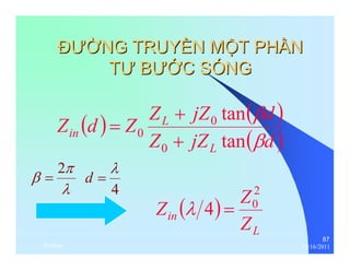
51. LC 2 [rad /m]
51
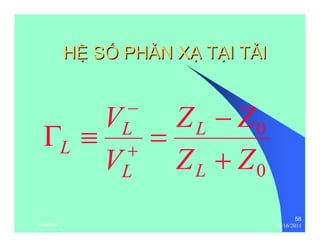
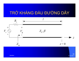
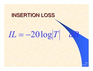
HẰẰNG SỐỐ SÓNG
π
λ
β =ω =
thenhan 12/16/2011

52. 52
thenhan 12/16/2011

53. 53
i(z,t)
I (z)
S V L Z
z l
v(z,t)
V (z)
MÔ HÌNH MẠẠCH ĐĐƯƯỜỜNG DÂY DÀI
S Z
+
-
0
thenhan 12/16/2011

54. 54
PHƯƯƠƠNG TRÌNH TRUYỀỀN SÓNG
TRÊN ĐĐƯƯỜỜNG DÂY
thenhan 12/16/2011

55. 55
TRỞỞ KHÁNG ĐĐẶẶC TÍNH CỦỦA
ĐĐƯƯỜỜNG DÂY 0 Z
thenhan 12/16/2011

56. 56
TẢẢI TRÊN ĐĐƯƯỜỜNG DÂY
TRUYỀỀN SÓNG
thenhan 12/16/2011

57. 57
+
V0
S V L Z
+
-
HỆỆ SỐỐ PHẢẢN XẠẠ
S Z
z
l
−
V0
Z0 ,β
d
thenhan 12/16/2011
PS
( ) + − j β d
− j β d
Ii z = I 0 e Ir ( z ) = I 0
e ( ) j d
Vi z V e = + − β 0
( ) j d
Vr z V e = − β 0
−
VL
+|L
V

58. 58
HỆỆ SỐỐ PHẢẢN XẠẠ TẠẠI TẢẢI
0
0
Z Z
L
−
−
Γ ≡ = +
L +
Z Z
V
V
L
L
L
thenhan 12/16/2011

59. Γ d = V d = Γ • −2 β
j d
59
HỆỆ SỐỐ PHẢẢN XẠẠ TẠẠI MỘỘT ĐĐiỂỂM
TRÊN ĐĐƯƯỜỜNG DÂY
( ) ( )
r e
V ( d
)
L
i
d = l − z
thenhan 12/16/2011

60. 60
HỆỆ SỐỐ PHẢẢN XẠẠ CÔNG SUẤẤT
+
-
Z0 ,β
thenhan 12/16/2011
S Z
S V L Z
z
l
+
V0
−
V0
d
Pi (z)
Pr (z)
Pi (l)
Pr (l)
PL
PS
Pi (0)
Pr (0)

61. 61
HỆỆ SỐỐ PHẢẢN XẠẠ CÔNG SUẤẤT
P
i
2 ( )2 d
Γ = r = Γ
P
thenhan 12/16/2011

62. 62
CÁC TRƯƯỜỜNG HỢỢP ĐĐẶẶC BIỆỆT
TẢẢI NGẮẮN MẠẠCH
Z R
L
0
L
−
Γ =
L +
Z R
0
1
0
0
R
0 = −
R
0
Vi (l) = −Vr (l)
V(l) = Vi (l)+Vr (l) = 0
−
+
=
ΓL
thenhan 12/16/2011

63. 63
Z0 ,β
thenhan 12/16/2011
+
-
TRỞỞ KHÁNG ĐĐƯƯỜỜNG DÂY
S Z
S V L Z
d l
Z(d )
ZIN

64. Z d Z Z jZ β
d
( )Ω
64
TRỞỞ KHÁNG TẠẠI ĐĐiỂỂM CÁCH TẢẢI
MỘỘT KHOẢẢNG d
( ) L
+
0
tan
( )
Z +
jZ d
=
L
β
tan
0
0
thenhan 12/16/2011

65. 65
TRỞỞ KHÁNG ĐĐẦẦU ĐĐƯƯỜỜNG DÂY
thenhan 12/16/2011

66. 66
thenhan 12/16/2011

67. 67
STANDING WAVE
thenhan 12/16/2011

68. 68
thenhan 12/16/2011

69. 69
thenhan 12/16/2011

70. 70
thenhan 12/16/2011

71. 71
TỈỈ SỐỐ SÓNG ĐĐỨỨNG LỚỚN
thenhan 12/16/2011

72. 72
thenhan 12/16/2011

73. 73
TỈỈ SỐỐ SÓNG ĐĐỨỨNG NHỎỎ
thenhan 12/16/2011

74. 74
SÓNG ĐĐỨỨNG TRÊN ĐĐƯƯỜỜNG
DÂY
TỈỈ SỐỐ SÓNG ĐĐỨỨNG
VSWR = V
max
V
min
thenhan 12/16/2011

75. 75
thenhan 12/16/2011

76. 76
thenhan 12/16/2011

77. 77
thenhan 12/16/2011

78. 78
thenhan 12/16/2011

79. 79
thenhan 12/16/2011

80. 80
thenhan 12/16/2011

81. 81
thenhan 12/16/2011

82. 82
thenhan 12/16/2011

83. 83
thenhan 12/16/2011

84. 84
thenhan 12/16/2011

85. 85
CÁC TRƯƯỜỜNG HỢỢP ĐĐẶẶT BIỆỆT
z ĐƯỜNG DÂY NGẮN
MẠCH TẢI
( ) ( )
+
β
Z d Z Z L
jZ 0
tan
d
Z jZ ( d )
=
in β
L
tan
0 +
0
Zin (d ) jZ ( d ) 0 tan β =
= 0 ZL
thenhan 12/16/2011

86. 86
CÁC TRƯƯỜỜNG HỢỢP ĐĐẶẶT BIỆỆT
z ĐƯỜNG DÂY HỞ
MẠCH TẢI
( ) ( )
+
β
Z d Z Z L
jZ 0
tan
d
Z jZ ( d )
=
in β
L
tan
0 +
0
Zin (d ) jZ ( d ) 0 cotan β = −
= ∞ ZL
thenhan 12/16/2011

87. 87
ĐĐƯƯỜỜNG TRUYỀỀN MỘỘT PHẦẦN
TƯƯ BƯƯỚỚC SÓNG
( ) ( )
+
β
Z d Z Z L
jZ 0
tan
d
Z jZ ( d )
=
in β
L
tan
0 +
0
Z ( )
Z
2
λ 4 = 0
L
in Z
β = 2
π
λ
λ
4
d =
thenhan 12/16/2011

88. 88
z DÂY NGẮN MẠCH:
(λ 4) = ∞ ZIN
= 0 ZL
z DÂY HỞ MẠCH:
(λ 4) = 0 ZIN
= ∞ ZL
thenhan 12/16/2011

89. 89
z DÂY NGẮN MẠCH:
(λ 4) = ∞ ZIN
= 0 ZL
z DÂY HỞ MẠCH:
(λ 4) = 0 ZIN
= ∞ ZL
thenhan 12/16/2011

90. 90
Frequency Dielectric Comments and history
"Bayonet type-N connector", or "Bayonet Neill-
Concelman" according to Johnson
Components. Developed in the early 1950s
at Bell Labs. Could also stand for "baby N
connector".
"Sub-miniature type B", a snap-on subminiature
connector, available in 50 and 75 ohms.
Limit
Connector type
BNC 4 GHz PTFE
SMB 4 GHz PTFE
OSMT 6 GHz PTFE A surface mount connector
MCX was the original name of the Snap-
On"micro-coax" connector species. Available
in 50 and 75 ohms.
Micro-miniature coax connector, popular in the
wire industry because its small size and
cheap price.
Sub-miniature type C, a threaded subminiature
connector, not widely used.
Sub-miniature type A developed in the 1960s,
perhaps the most widely-used microwave
connector system in the universe.
"Threaded Neill-Concelman" connector,
according to Johnson Components, it is
actually a threaded BNC connector, to
reduce vibration problems. Carl Concelman
was an engineer at Amphenol.
OSX, MCX, PCX 6 GHz PTFE
MMCX PTFE
SMC 10 GHz PTFE
SMA 25 GHz PTFE
TNC 15 GHz PTFE
thenhan 12/16/2011

91. 91
Named for Paul Neill of Bell Labs in the 1940s,
available in 50 and 75 ohms. Cheap and
rugged, it is still widely in use. Originally was
usable up to one GHz, but over the years this
species has been extended to 18 GHz, including
work by Julius Botka at Hewlett Packard.
APC-7 stands for "Amphenol precision connector",
7mm. Developed in the swinging 60s, ironically
a truly sexless connector, which provides the
lowest VSWR of any connector up to 18 GHz.
OSP stands for "Omni-Spectra push-on", a blind-mate
connector with zero detent. Often used in
equipment racks.
A precision (expensive) connector, it mates to
cheaper SMA connectors.
OSP stands for "Omni-Spectra subminiature push-on",
a smaller version of OSP connector.
11 GHz PTFE
normal
18 GHz
precision
APC-7, 7 mm 18 GHz PTFE
OSP 22 GHz PTFE
3.5 mm 26.5 GHz Air
OSSP 28 GHz PTFE
SSMA 38 GHz PTFE Smaller than an SMA.
Precision connector, developed by Mario Maury in
1974. 2.92 mm will thread to cheaper SMA and
3.5 mm connectors. Often called "2.9 mm".
The original mass-marketed 2.92 mm connector,
made by Wiltron (now Anritsu). Named the "K"
connector, meaning it covers all of the K
frequency bands.
2.92 mm 40 GHz Air
K 40 GHz Air
thenhan 12/16/2011
N
"Threaded Neill-Concelman" connector, according to
Johnson Components, it is actually a threaded
BNC connector, to reduce vibration problems.
Carl Concelman was an engineer at Amphenol.
TNC 15 GHz PTFE

92. 92
"Gilbert push-on", "Omni-spectra microminiature
push-on"
GPO, OSMP, SMP 40 GHz PTFE
OS-50P 40 GHz Smaller version of OSP blind-mate connector.
2.4 mm, and 1.85 mm will mate with each other
without damage. Developed by Julius Botka and
Paul Watson in 1986, along with the 1.85 mm
connector.
2.4 mm 50 GHz Air
1.85 mm 60 GHz Air Mechanically compatible with 2.4 mm connectors.
Anritsu's term for 1.85 mm connectors because
they span the V frequency band.
The Rolls Royce of connectors. This connector
species works up to 110 GHz. It costs a fortune!
Developed at Hewlett Packard (now Agilent) by
Paul Watson in 1989.
V 60 GHz Air
1 mm 110 GHz Air
thenhan 12/16/2011

93. 93
thenhan 12/16/2011

94. 94
thenhan 12/16/2011

95. 95
thenhan 12/16/2011

96. 96
thenhan 12/16/2011

97. 97
thenhan 12/16/2011

98. 98
RETURN LOSS
RL = −20logΓ dB
thenhan 12/16/2011

99. 99
TRANSMISSION COEFICIENT
T =1+ Γ
T Z Z
0 1 2
Z
L
Z Z
L
+
=
0 0
L
−
Z Z
L
+
= +
thenhan 12/16/2011

100. 100
INSERTION LOSS
IL = −20logT dB
thenhan 12/16/2011

101. 101
SMITH CHART
thenhan 12/16/2011

102. 102
MỐỐI QUAN HỆỆ GIỮỮA TRỞỞ
KHÁNG VÀ HỆỆ SỐỐ PHẢẢN XẠẠ
( ) ( )
Z x Z x
(x)
+ Γ
− Γ
=
1
0
1
thenhan 12/16/2011

103. 103
CÁC GIÁ TRỊỊ CHUẨẨN HÓA
( ) ( )
z x = Z x
0 R
TRỞỞ KHÁNG CHUẦẦN HÓA
z = r + jx
thenhan 12/16/2011

104. 104
z ZL
L =
0 R
1
r R
0
0 = =
R
0
( ) ( )
y x = Y x
Y
0 Y ( x ) = 1
Z ( x
) thenhan 12/16/2011

105. 105
HỆỆ SỐỐ PHẢẢN XẠẠ
( ) ( )
x Z x R
0
−
Γ =
( ) ( )
( ) 0
Z x +
R
1
−
x Z x R
0
+
( ) 1
Z x R
0
Γ =
thenhan 12/16/2011

106. 106
MỐỐI QUAN HỆỆ GIỮỮA HỆỆ SỐỐ
PHẢẢN XẠẠ VÀ TRỞỞ KHÁNG
CHUẨẨN HÓA
1
+
1
−
x z x
Γ =
z x
thenhan 12/16/2011

107. 107
Γ(x) z(x)
z(x) Γ(x)
z CÓ 1 GIÁ TRỊ THÌ CHỈ CÓ DUY NHẤT 1 GIÁ TRỊ
z CÓ 1 GIÁ TRỊ THÌ CHỈ CÓ DUY NHẤT 1 GIÁ TRỊ
thenhan 12/16/2011

108. Γ(x) = 0.8∠600
108
BẢẢN CHẤẤT VÀ CÁCH BIỂỂU DIỂỂN
HỆỆ SỐỐ PHẢẢN XẠẠ
+1
Mặt phẳng phức
0.8
−1 +1
600
Γ(x)
Re(Γ(x))
Im(Γ)
Im(Γ(x))
Re(Γ)
0
−1
thenhan 12/16/2011

109. 109
HỆỆ SỐỐ PHẢẢN XẠẠ
(x) (x) j (x) r i Γ = Γ + Γ
r i Dạng đơn giản Γ = Γ + jΓ
⎧
Γ r
= Re
( Γ
)
⎨ ⎩ Γ i
= Im
( Γ
) thenhan 12/16/2011

110. 110
TRỞỞ KHÁNG ĐĐƯƯỜỜNG DÂY
Z(x) = R(x)+ jX (x)
Z = R + jX
thenhan 12/16/2011

111. 111
TRỞỞ KHÁNG CHUẨẨN HÓA
z(x) = r(x)+ jx
z = r + jx
r = R
0 R
x = X
0 R
Trở kháng đường
dây chuẩn hóa
Điện trở đường dây
chuẩn hóa
Điện kháng đường
dây chuẩn hóa
thenhan 12/16/2011

112. 112
r jx j
+ Γ + Γ
r i
j
− Γ − Γ
r i
+ =
1
1
thenhan 12/16/2011

113. 113
− Γ − Γ
2 2
1
r r i
( )2 2
1
− Γ + Γ
r i
=
2
Γ
x i
( 2 1
− Γ )+ Γ
2 r i
=
thenhan 12/16/2011

114. 114
PHƯƯƠƠNG TRÌNH ĐĐƯƯỜỜNG TRÒN
2
⎞
+ Γ 2
⎟⎠
= 2
⎛
+
r i
r r
1
1
1
⎞
⎟⎠
⎜⎝
⎛
⎜⎝
r
+
Γ −
⎞
⎟⎠
r
⎛
+
⎜⎝
0 ,
1 r
tâm
bán kính
1
1+ r
thenhan 12/16/2011

115. 115
Re(Γ)
Im(Γ)
i Γ
+1
Mặt phẳng phức
r = 0
r = 0.2
r = 0.5
−1 r =1 r = 2
+1
−1
0
r Γ
thenhan 12/16/2011

116. 116
PHƯƯƠƠNG TRÌNH ĐĐƯƯỜỜNG TRÒN
2 2
( )
2 1 1 ⎛ 1 ⎞
⎟⎠
= ⎟⎠
⎜⎝
⎞
Γ − + ⎛Γ −
⎜⎝
x x r i
⎞
⎟⎠
1, 1 tâm
⎛
x
⎜⎝
bán kính
1
x
thenhan 12/16/2011

117. 117
Re(Γ)
Im(Γ)
i Γ
+1
Mặt phẳng phức
x = 0.5 x =1
−1 +1
x = −0.5 x = −1
−1
0
r Γ
thenhan 12/16/2011

118. 118
Re(Γ)
Im(Γ)
i Γ
+1
Mặt phẳng phức
x = 0.5 x =1
−1 +1
x = −1
−1
0
r Γ
x = −0.5
thenhan 12/16/2011

119. 119
Re(Γ)
Im(Γ)
i Γ
+1
Mặt phẳng phức
r = 0
r = 0.2
r = 0.5
−1 r =1 r = 2
+1
−1
0
r Γ
thenhan 12/16/2011

120. 120
Re(Γ)
Im(Γ)
i Γ
+1
Mặt phẳng phức
x = 0.5
x =1
r = 0.2
r = 0.5
−1 +1
r =1 r = 2
x = −1
−1
0
r Γ
x = −0.5
thenhan 12/16/2011

121. 121
thenhan 12/16/2011

122. 122
thenhan 12/16/2011

123. 123
thenhan 12/16/2011

124. 124
thenhan 12/16/2011

125. 125
thenhan 12/16/2011

126. 126
thenhan 12/16/2011

127. 127
ỨỨng dụụng củủa đđồồ thịị SMITH
thenhan 12/16/2011