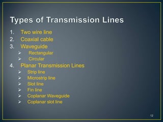
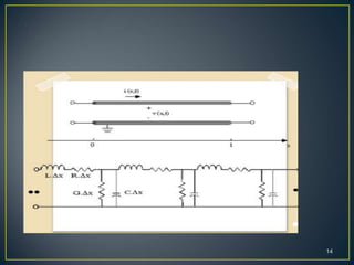
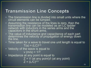
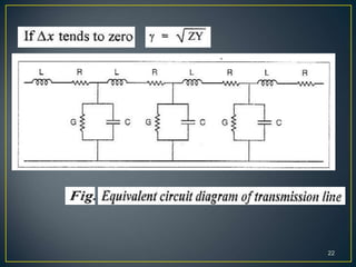
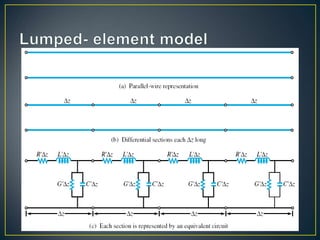
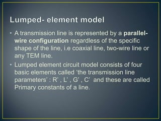
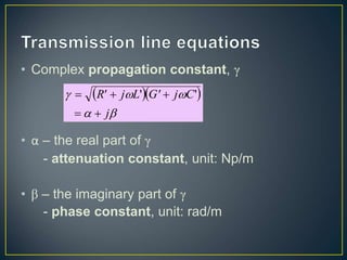
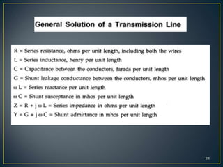
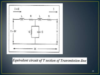
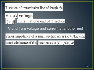
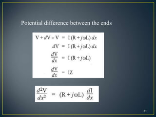
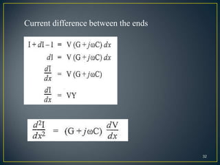
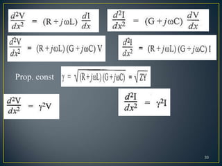
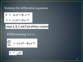
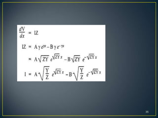
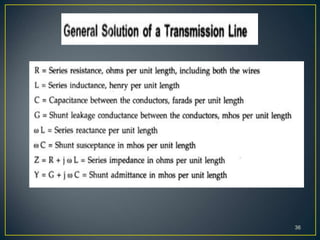
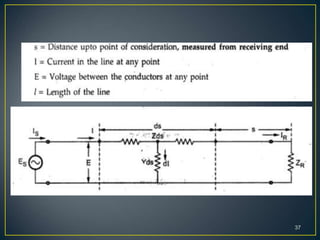
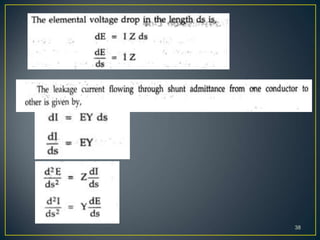
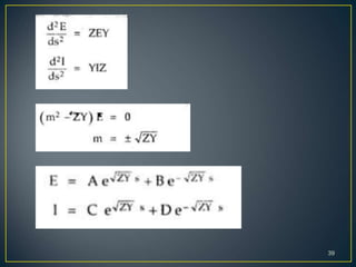
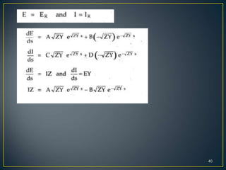
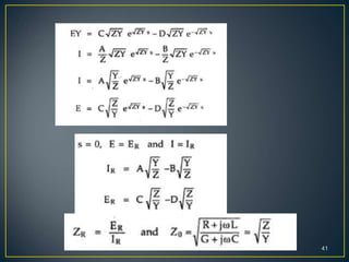
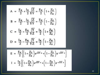
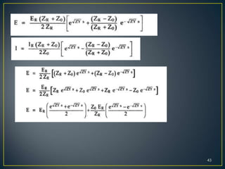
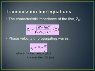
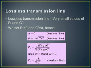
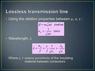
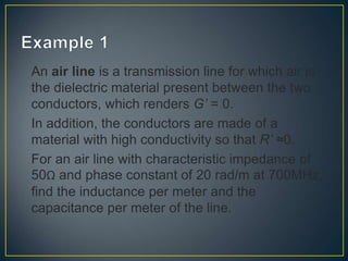
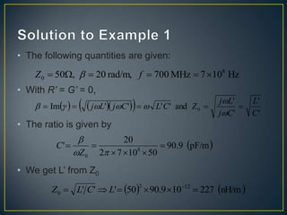
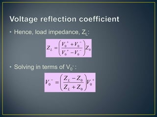
1
SRI RAMAKRISHNA INSTITUTE OF TECHNOLOGY
(An Autonomous Institution)
(Approved by AICTE-New Delhi, Affiliated to Anna University-Chennai)
(NAAC Accredited Institution with “A” Grade)
Pachapalayam, Perur Chettipalayam,Coimbatore,Tamilnadu-641010.
DEPARTMENT OF ELECTRONICS AND COMMUNICATION ENGINEERING
20EC009 – TRANSMISSION LINES
AND WAVEGUIDES
Ms.R.Kanmani
Assistant Professor (Sr.Gr)
Department of ECE
20EC009 TRANSMISSION LINES AND WAVE
GUIDES
L T P C
3 0 0 3
The course will enable the students to learn about the
transmission line parameters, characteristics of High
Frequency Transmission lines, impedance matching
techniques, Smith chart, and characteristics of waves between
parallel plates and in waveguides.
OBJECTIVES:
2
UNIT I
Transmission Lines Parameters
A line of cascaded T sections- General solution of
transmission lines- Physical significance of the
equations, infinite line, wavelength, velocity of
propagation, distortion line- reflection on a line not
terminated in Zo, reflection coefficient, open and
short circuited lines, insertion loss, input impedance,
transfer impedance.
3
UNIT II
The Line at Radio Frequency
Parameter of the open wire line and coaxial line at
RF- Line constants for dissipation less line, voltages
and currents on the dissipation less line, standing
waves, input impedance of open and short circuited
lines- power and impedance measurement on lines.
4
UNIT III
Line Impedance Matching Techniques and Smith
Chart
λ/2, λ/4, λ/8 line- Quarter Wave line impedance
matching- single and double stub matching, Smith
chart and its applications, problem solving using
Smith chart, numerical tools.
5
UNIT IV
Parallel Planes and Rectangular Waveguide
General solutions for TE and TM waves, Waves between
parallel plates of perfect conductors Velocities of wave
propagation- Attenuation in parallel plate waveguide, Wave
impedance of TE and TM waves in a parallel plate
waveguide, Characteristics of TE and TM waves –
Impossibility of TEM waves in rectangular waveguides,
Dominant mode, Wave impedances of TE and TM waves,
Characteristic impedance of a waveguide – Attenuation
factor, Excitation of various modes.
6
UNIT V
Circular Waveguides and Cavity Resonators
Bessel functions, TE and TM modes in circular
waveguides- wave impedances, dominant mode,
excitation of mode- Microwave cavity resonators,
rectangular and Circular cavity resonators- Q factor
of a rectangular cavity resonator for the TE101
mode.
7
COURSE OUTCOMES:
• CO1:Ability to understand the concepts of wave
propagation in Transmission line and waveguide.
• CO2:Ability to analyze the wave propagation in
transmission line and waveguide.
• CO3:Ability to determine various line parameters for the
specified transmission line.
• CO4:Ability to determine waveguide parameters for the
different modes of propagation.
• CO5:Ability to design stub and quarter wave line
matching circuits.
8
9
REFERENCES:
1. Ryder J.D, “Networks, Lines and Fields”, 2nd Edition,
Prentice Hall of India, New Delhi, 2015.
2. Jordan E.C, “Electromagnetic Waves and Radiating
Systems”, Prentice Hall of India, 2015.
3. B. Somanathan Nair, “Transmission Lines and Wave
guides”, Sanguine Technical Publishers, 2006.
4. G.S.N Raju, “Electromagnetic Field Theory and
Transmission Lines”, Pearson Education, 1st Edition, 2005.
5. W.H.Hayt, ”Engineering Electromagnetics”, 9th edition,
McGraw Hill, 2020.
10
UNIT 1
• Introduction:
• Transmission Line is a structure which can transport
electrical energy from one point to another.
• In an electronic system, the delivery of power
requires the connection of two wires between the source
and the load. At low frequencies, power is considered to
be delivered to the load through the wire.
• In the microwave frequency region, power is
considered to be in electric and magnetic fields that are
guided from place to place by some physical structure.
Any physical structure that will guide an electromagnetic
wave place to place is called a Transmission Line.
11
1. Two wire line
2. Coaxial cable
3. Waveguide
 Rectangular
 Circular
4. Planar Transmission Lines
 Strip line
 Microstrip line
 Slot line
 Fin line
 Coplanar Waveguide
 Coplanar slot line
12
 Has two conductors running parallel
 Can propagate a signal at any frequency (in theory)
 Becomes lossy at high frequency
 Can handle low or moderate amounts of power
 Does not have signal distortion, unless there is loss
 May or may not be immune to interference
 Does not have Ez or Hz components of the fields (TEMz)
13
14
• The transmission line is divided into small units where the
circuit elements can be lumped.
• Assuming the resistance of the lines is zero, then the
transmission line can be modeled as an LC ladder
network with inductors in the series arms and the
capacitors in the shunt arms.
• The value of inductance and capacitance of each part
determines the velocity of propagation of energy down
the line.
• Time taken for a wave to travel one unit length is equal to
T(s) = (LC)0.5
• Velocity of the wave is equal to
v (m/s) = 1/T
• Impedance at any point is equal to
Z = V (at any point)/I (at any point)
Z = (L/C)0.5
15
• Line terminated in its characteristic impedance: If the
end of the transmission line is terminated in a resistor
equal in value to the characteristic impedance of the line
as calculated by the formula Z=(L/C)0.5 , then the voltage
and current are compatible and no reflections occur.
• Line terminated in a short: When the end of the
transmission line is terminated in a short (RL = 0), the
voltage at the short must be equal to the product of the
current and the resistance.
• Line terminated in an open: When the line is terminated
in an open, the resistance between the open ends of the
line must be infinite. Thus the current at the open end is
zero.
16
17
18
19
20
21
22
• A transmission line is represented by a parallel-
wire configuration regardless of the specific
shape of the line, i.e coaxial line, two-wire line or
any TEM line.
• Lumped element circuit model consists of four
basic elements called ‘the transmission line
parameters’ : R’ , L’ , G’ , C’ and these are called
Primary constants of a line.
• Lumped-element transmission line parameters:
• R’ : combined resistance of both conductors per unit length, in Ω/m
• L’ : the combined inductance of both conductors per unit length, in
H/m
• G’ : the conductance of the insulation medium per unit length, in
S/m
• C’ : the capacitance of the two conductors per unit length, in F/m
• Complex propagation constant, γ
• α – the real part of γ
- attenuation constant, unit: Np/m
• β – the imaginary part of γ
- phase constant, unit: rad/m
  





j
C
j
G'
L
j
R'




 '
'
27
28
29
30
V and I are voltage and current at another end
31
Potential difference between the ends
32
Current difference between the ends
33
Prop. const
34
Solution for differential equations
Differentiating w.r t x
35
36
37
38
39
40
41
42
43
44
45
• The characteristic impedance of the line, Z0 :
• Phase velocity of propagating waves:
where f = frequency (Hz)
λ = wavelength (m)
 




'
'
'
'
0
C
j
G
L
j
R
Z




 
 f
up
• Lossless transmission line - Very small values of
R’ and G’.
• We set R’=0 and G’=0, hence:
line)
(lossless
'
'
line)
(lossless
0
C
L





line)
(lossless
'
'
0,
G'
and
0
R'
since
'
'
'
'
0
0
C
L
Z
C
j
G
L
j
R
Z








• Using the relation properties between μ, σ, ε :
• Wavelength, λ
Where εr = relative permittivity of the insulating
material between conductors
(m/s)
1
(rad/m)






p
u
r
r
p
f
c
f
u



 0
1



An air line is a transmission line for which air is
the dielectric material present between the two
conductors, which renders G’ = 0.
In addition, the conductors are made of a
material with high conductivity so that R’ ≈0.
For an air line with characteristic impedance of
50Ω and phase constant of 20 rad/m at 700MHz,
find the inductance per meter and the
capacitance per meter of the line.
• The following quantities are given:
• With R’ = G’ = 0,
• The ratio is given by
• We get L’ from Z0
Hz
10
7
MHz
700
rad/m,
20
,
50 8
0 




 f
Z 
    
  '
'
'
'
and
'
'
'
'
Im 0
C
L
C
j
L
j
Z
C
L
C
j
L
j 











 
pF/m
9
.
90
50
10
7
2
20
' 8
0









Z
C
   
nH/m
227
10
9
.
90
50
'
'
' 12
2
0 




 
L
C
L
Z
• The load impedance, ZL
Where;
= total voltage at the load
V0
- = amplitude of reflected voltage wave
V0
+ = amplitude of the incident voltage wave
= total current at the load
Z0 = characteristic impedance of the line



 0
0
~
V
V
VL
L
V
~
0
0
0
0
~
Z
V
Z
V
IL




L
I
~
L
L
L
I
V
Z ~
~

• Hence, load impedance, ZL:
• Solving in terms of V0
- :
0
0
0
0
0
Z
V
V
V
V
ZL 









 















 0
0
0
0 V
Z
Z
Z
Z
V
L
L
• Voltage reflection coefficient, Γ – the ratio of the
amplitude of the reflected voltage wave, V0
- to the
amplitude of the incident voltage wave, V0
+ at the
load.
• Hence,
less)
(dimension
1
1
0
0
0
0
0
0







 

Z
Z
Z
Z
Z
Z
Z
Z
V
V
L
L
L
L
• Z0 for lossless line is a real number while ZL in
general is a complex number. Hence,
Where |Γ| = magnitude of Γ
θr = phase angle of Γ
• A load is matched to the line if ZL = Z0 because
there will be no reflection by the load (Γ = 0 and
V0
−= 0.
r
j
e 



• The load impedance, ZL
Where;
= total voltage at the load
V0
- = amplitude of reflected voltage wave
V0
+ = amplitude of the incident voltage wave
= total current at the load
Z0 = characteristic impedance of the line



 0
0
~
V
V
VL
L
V
~
0
0
0
0
~
Z
V
Z
V
IL




L
I
~
L
L
L
I
V
Z ~
~

• A 100-Ω transmission line is connected to a load
consisting of a 50-Ω resistor in series with a 10pF
capacitor. Find the reflection coefficient at the
load for a 100-MHz signal.
• The following quantities are given
• The load impedance is
• Voltage reflection coefficient is
Hz
10
MHz
100
,
100
F,
10
,
50 8
0
11
L
L 





 
f
Z
C
R
 









159
50
10
10
2
1
50
/
11
8
L
L
L
j
j
C
j
R
Z














 7
.
60
76
.
0
1
59
.
1
5
.
0
1
59
.
1
5
.
0
1
/
1
/
0
L
0
L
j
j
Z
Z
Z
Z
58
The ordinary telephone cable is an underground
cable which consists of wires insulated with
paper and twisted in pair. For the audio
frequency range, the inductance L and
conductance G of such a cable is negligibly
small and hence can be neglected. Hence
impedance and admittance of such a cable
becomes,
59
60
61
62

TLW_Unit I material pdf.ppt

  • 1.
    1 SRI RAMAKRISHNA INSTITUTEOF TECHNOLOGY (An Autonomous Institution) (Approved by AICTE-New Delhi, Affiliated to Anna University-Chennai) (NAAC Accredited Institution with “A” Grade) Pachapalayam, Perur Chettipalayam,Coimbatore,Tamilnadu-641010. DEPARTMENT OF ELECTRONICS AND COMMUNICATION ENGINEERING 20EC009 – TRANSMISSION LINES AND WAVEGUIDES Ms.R.Kanmani Assistant Professor (Sr.Gr) Department of ECE
  • 2.
    20EC009 TRANSMISSION LINESAND WAVE GUIDES L T P C 3 0 0 3 The course will enable the students to learn about the transmission line parameters, characteristics of High Frequency Transmission lines, impedance matching techniques, Smith chart, and characteristics of waves between parallel plates and in waveguides. OBJECTIVES: 2
  • 3.
    UNIT I Transmission LinesParameters A line of cascaded T sections- General solution of transmission lines- Physical significance of the equations, infinite line, wavelength, velocity of propagation, distortion line- reflection on a line not terminated in Zo, reflection coefficient, open and short circuited lines, insertion loss, input impedance, transfer impedance. 3
  • 4.
    UNIT II The Lineat Radio Frequency Parameter of the open wire line and coaxial line at RF- Line constants for dissipation less line, voltages and currents on the dissipation less line, standing waves, input impedance of open and short circuited lines- power and impedance measurement on lines. 4
  • 5.
    UNIT III Line ImpedanceMatching Techniques and Smith Chart λ/2, λ/4, λ/8 line- Quarter Wave line impedance matching- single and double stub matching, Smith chart and its applications, problem solving using Smith chart, numerical tools. 5
  • 6.
    UNIT IV Parallel Planesand Rectangular Waveguide General solutions for TE and TM waves, Waves between parallel plates of perfect conductors Velocities of wave propagation- Attenuation in parallel plate waveguide, Wave impedance of TE and TM waves in a parallel plate waveguide, Characteristics of TE and TM waves – Impossibility of TEM waves in rectangular waveguides, Dominant mode, Wave impedances of TE and TM waves, Characteristic impedance of a waveguide – Attenuation factor, Excitation of various modes. 6
  • 7.
    UNIT V Circular Waveguidesand Cavity Resonators Bessel functions, TE and TM modes in circular waveguides- wave impedances, dominant mode, excitation of mode- Microwave cavity resonators, rectangular and Circular cavity resonators- Q factor of a rectangular cavity resonator for the TE101 mode. 7
  • 8.
    COURSE OUTCOMES: • CO1:Abilityto understand the concepts of wave propagation in Transmission line and waveguide. • CO2:Ability to analyze the wave propagation in transmission line and waveguide. • CO3:Ability to determine various line parameters for the specified transmission line. • CO4:Ability to determine waveguide parameters for the different modes of propagation. • CO5:Ability to design stub and quarter wave line matching circuits. 8
  • 9.
    9 REFERENCES: 1. Ryder J.D,“Networks, Lines and Fields”, 2nd Edition, Prentice Hall of India, New Delhi, 2015. 2. Jordan E.C, “Electromagnetic Waves and Radiating Systems”, Prentice Hall of India, 2015. 3. B. Somanathan Nair, “Transmission Lines and Wave guides”, Sanguine Technical Publishers, 2006. 4. G.S.N Raju, “Electromagnetic Field Theory and Transmission Lines”, Pearson Education, 1st Edition, 2005. 5. W.H.Hayt, ”Engineering Electromagnetics”, 9th edition, McGraw Hill, 2020.
  • 10.
  • 11.
    • Introduction: • TransmissionLine is a structure which can transport electrical energy from one point to another. • In an electronic system, the delivery of power requires the connection of two wires between the source and the load. At low frequencies, power is considered to be delivered to the load through the wire. • In the microwave frequency region, power is considered to be in electric and magnetic fields that are guided from place to place by some physical structure. Any physical structure that will guide an electromagnetic wave place to place is called a Transmission Line. 11
  • 12.
    1. Two wireline 2. Coaxial cable 3. Waveguide  Rectangular  Circular 4. Planar Transmission Lines  Strip line  Microstrip line  Slot line  Fin line  Coplanar Waveguide  Coplanar slot line 12
  • 13.
     Has twoconductors running parallel  Can propagate a signal at any frequency (in theory)  Becomes lossy at high frequency  Can handle low or moderate amounts of power  Does not have signal distortion, unless there is loss  May or may not be immune to interference  Does not have Ez or Hz components of the fields (TEMz) 13
  • 14.
  • 15.
    • The transmissionline is divided into small units where the circuit elements can be lumped. • Assuming the resistance of the lines is zero, then the transmission line can be modeled as an LC ladder network with inductors in the series arms and the capacitors in the shunt arms. • The value of inductance and capacitance of each part determines the velocity of propagation of energy down the line. • Time taken for a wave to travel one unit length is equal to T(s) = (LC)0.5 • Velocity of the wave is equal to v (m/s) = 1/T • Impedance at any point is equal to Z = V (at any point)/I (at any point) Z = (L/C)0.5 15
  • 16.
    • Line terminatedin its characteristic impedance: If the end of the transmission line is terminated in a resistor equal in value to the characteristic impedance of the line as calculated by the formula Z=(L/C)0.5 , then the voltage and current are compatible and no reflections occur. • Line terminated in a short: When the end of the transmission line is terminated in a short (RL = 0), the voltage at the short must be equal to the product of the current and the resistance. • Line terminated in an open: When the line is terminated in an open, the resistance between the open ends of the line must be infinite. Thus the current at the open end is zero. 16
  • 17.
  • 18.
  • 19.
  • 20.
  • 21.
  • 22.
  • 24.
    • A transmissionline is represented by a parallel- wire configuration regardless of the specific shape of the line, i.e coaxial line, two-wire line or any TEM line. • Lumped element circuit model consists of four basic elements called ‘the transmission line parameters’ : R’ , L’ , G’ , C’ and these are called Primary constants of a line.
  • 25.
    • Lumped-element transmissionline parameters: • R’ : combined resistance of both conductors per unit length, in Ω/m • L’ : the combined inductance of both conductors per unit length, in H/m • G’ : the conductance of the insulation medium per unit length, in S/m • C’ : the capacitance of the two conductors per unit length, in F/m
  • 26.
    • Complex propagationconstant, γ • α – the real part of γ - attenuation constant, unit: Np/m • β – the imaginary part of γ - phase constant, unit: rad/m         j C j G' L j R'      ' '
  • 27.
  • 28.
  • 29.
  • 30.
    30 V and Iare voltage and current at another end
  • 31.
  • 32.
  • 33.
  • 34.
    34 Solution for differentialequations Differentiating w.r t x
  • 35.
  • 36.
  • 37.
  • 38.
  • 39.
  • 40.
  • 41.
  • 42.
  • 43.
  • 44.
  • 45.
  • 46.
    • The characteristicimpedance of the line, Z0 : • Phase velocity of propagating waves: where f = frequency (Hz) λ = wavelength (m)       ' ' ' ' 0 C j G L j R Z        f up
  • 47.
    • Lossless transmissionline - Very small values of R’ and G’. • We set R’=0 and G’=0, hence: line) (lossless ' ' line) (lossless 0 C L      line) (lossless ' ' 0, G' and 0 R' since ' ' ' ' 0 0 C L Z C j G L j R Z        
  • 48.
    • Using therelation properties between μ, σ, ε : • Wavelength, λ Where εr = relative permittivity of the insulating material between conductors (m/s) 1 (rad/m)       p u r r p f c f u     0 1   
  • 49.
    An air lineis a transmission line for which air is the dielectric material present between the two conductors, which renders G’ = 0. In addition, the conductors are made of a material with high conductivity so that R’ ≈0. For an air line with characteristic impedance of 50Ω and phase constant of 20 rad/m at 700MHz, find the inductance per meter and the capacitance per meter of the line.
  • 50.
    • The followingquantities are given: • With R’ = G’ = 0, • The ratio is given by • We get L’ from Z0 Hz 10 7 MHz 700 rad/m, 20 , 50 8 0       f Z         ' ' ' ' and ' ' ' ' Im 0 C L C j L j Z C L C j L j               pF/m 9 . 90 50 10 7 2 20 ' 8 0          Z C     nH/m 227 10 9 . 90 50 ' ' ' 12 2 0        L C L Z
  • 51.
    • The loadimpedance, ZL Where; = total voltage at the load V0 - = amplitude of reflected voltage wave V0 + = amplitude of the incident voltage wave = total current at the load Z0 = characteristic impedance of the line     0 0 ~ V V VL L V ~ 0 0 0 0 ~ Z V Z V IL     L I ~ L L L I V Z ~ ~ 
  • 52.
    • Hence, loadimpedance, ZL: • Solving in terms of V0 - : 0 0 0 0 0 Z V V V V ZL                             0 0 0 0 V Z Z Z Z V L L
  • 53.
    • Voltage reflectioncoefficient, Γ – the ratio of the amplitude of the reflected voltage wave, V0 - to the amplitude of the incident voltage wave, V0 + at the load. • Hence, less) (dimension 1 1 0 0 0 0 0 0           Z Z Z Z Z Z Z Z V V L L L L
  • 54.
    • Z0 forlossless line is a real number while ZL in general is a complex number. Hence, Where |Γ| = magnitude of Γ θr = phase angle of Γ • A load is matched to the line if ZL = Z0 because there will be no reflection by the load (Γ = 0 and V0 −= 0. r j e    
  • 55.
    • The loadimpedance, ZL Where; = total voltage at the load V0 - = amplitude of reflected voltage wave V0 + = amplitude of the incident voltage wave = total current at the load Z0 = characteristic impedance of the line     0 0 ~ V V VL L V ~ 0 0 0 0 ~ Z V Z V IL     L I ~ L L L I V Z ~ ~ 
  • 56.
    • A 100-Ωtransmission line is connected to a load consisting of a 50-Ω resistor in series with a 10pF capacitor. Find the reflection coefficient at the load for a 100-MHz signal.
  • 57.
    • The followingquantities are given • The load impedance is • Voltage reflection coefficient is Hz 10 MHz 100 , 100 F, 10 , 50 8 0 11 L L         f Z C R            159 50 10 10 2 1 50 / 11 8 L L L j j C j R Z                7 . 60 76 . 0 1 59 . 1 5 . 0 1 59 . 1 5 . 0 1 / 1 / 0 L 0 L j j Z Z Z Z
  • 58.
    58 The ordinary telephonecable is an underground cable which consists of wires insulated with paper and twisted in pair. For the audio frequency range, the inductance L and conductance G of such a cable is negligibly small and hence can be neglected. Hence impedance and admittance of such a cable becomes,
  • 59.
  • 60.
  • 61.
  • 62.