This document provides an overview of key concepts and measurement techniques in hydrometry. It covers topics such as network design, site selection, measurement frequency, and methods for measuring streamflow and water levels. A variety of equipment options are presented for recording stage, including staff gauges, wire gauges, bubblers and pressure transducers. Streamflow measurement methods like current meters, acoustic Doppler profilers and the slope-area technique are also described. The document establishes standard practices and terminology for surface water measurement in India.

![Design Manual – Hydrometry (SW) Volume 4
• Once the network density has been specified the sites for the water levels and discharges have to
be selected. Criteria for site selection are discussed in Chapter 4.
• Next, in Chapter 5 the observation frequency to be applied for the various hydrological quantities
in view of the measurement objectives and temporal variation of the observed processes are
treated.
• The measurement techniques for observation of hydrometric variables and related equipment are
dealt with in Chapter 6.
• Since the buyers of the hydrometric equipment are often neither sufficiently familiar with the exact
functioning of (parts of) the equipment nor with the background of the specifications, remarks on
the equipment specifications have been added in Chapter 7. The equipment specifications proper
are covered in a separate and regularly updated volume: “Equipment Specification Surface
Water”.
• Guidelines on station design and equipment installation are dealt with in Chapter 8.
In the Field Manual operational practices in running the network stations are given. It also includes
field inspections, audits and last but not least, the topic of equipment maintenance and calibration.
Notes
• The content of this part of the manual deals only with hydrometric measurements in the States of
Peninsular India. The equipment discussed is used or appropriate for use in the Hydrological
Information System. Hence, the manual does not provide a complete review of all techniques and
equipment applied elsewhere.
• The procedures dealt with in this manual are conformably to BIS and ISO standards. It is
essential that the procedures described in this manual are closely followed to guarantee a
standardised approach in the entire operation of the Hydrological Information System.
1.2 DEFINITION OF VARIABLES AND UNITS
In this section definitions, symbols and units of relevant quantities and parameters when dealing with
hydrometry are given. The use of standard methods is an important objective in the operation of the
Hydrological Information System (HIS). Standard methods require the use of a coherent system of
units with which variables and parameters are quantified. This section deals with the system of units
used for the measurement of hydrological quantities.
Quantity Symbol Unit Quantity Symbol Unit
Density
Density of water
Density of sediment,
Relative density under water
Pressure
Air pressure
Water pressure
Temperature
Water temperature
Air temperature
Level, depth, area
Water depth
Wetted perimeter
Wetted area
Hydraulic radius
Equilibrium or normal depth
Critical depth
ρ
ρs
Δ=(ρs-ρ)/ρ
pa
p
Tw ,tw
Ta ,ta
y, h
P
A
R
yn, hn
yc, hc
kg.m-3
kg.m-3
[-]
kPa
kPa
oC or K
oC or K
m
m
m2
m
m
m
Head
Velocity head
Pressure head
Energy head
Slope
Slope/gradient (general)
Bottom/bed slope/gradient
Water surface slope/gradient
Energy slope/gradient
Discharge
Flow velocity
Discharge
Discharge per unit width
Characteristic numbers
Reynolds number
Froude number
hv
hp
He
S
S0
Sw
Se
u, v, w
Q
q
Re
Fr
m
m
m
[-]
[-]
[-]
[-]
m.s-1
m3.s-1
m2.s-1
[-]
[-]
Table 1.1: Overview of relevant quantities, symbols and units used in hydrometry
Hydrometry January 2003 Page 2](https://image.slidesharecdn.com/swvolume4designmanualhydrometry-140924050537-phpapp02/85/Hydrometry-Design-Manual-Volume-4-2003-6-320.jpg)
![Design Manual – Hydrometry (SW) Volume 4
General terms
Control: The physical properties of a channel, natural or artificial, which determine the relationship
between stage and discharge at a location in the channel.
Stable channel: Channel in which the bed and the sides remain sensibly stable over a substantial
period of time in the control reach and in which scour and deposition during the rising and
falling floods is inappreciable.
Unstable channel: Channel in which there is frequently and significantly changing control.
Reach: A length of open channel between two defined cross-sections
Invert: The lowest part of the cross-section of a natural or artificial channel.
Wetted perimeter, P [m]: The wetted boundary of an open channel at a specified section.
Cross-section of stream, A [m2]: A specified section of the stream normal to the direction of flow
bounded by the wetted perimeter and the free water surface.
Hydraulic radius, R [m]: The quotient of the wetted cross-sectional area and the wetted perimeter.
Level, depth and gradient
Stage, y, h [m]: Height of water surface of a stream, river, lake or reservoir at the measuring point
above an established datum plane.
Gauge height, h [m]: Water surface elevation relative to the gauge datum.
Water depth D, h [m]: Vertical distance between water surface and river bottom.
Normal/equilibrium depth, [m]: Flow depth under steady, uniform flow conditions.
Critical depth, [m]: The depth of flow when the flow is critical (Fr = 1), see Chapter 2.
Gauge: The device installed at the gauging station for measuring the level of the water surface
relative to datum. If the gauge is linked to a standard system of levels then the gauge is a
reference gauge.
Water level recorder: A device which records automatically, either continuously or at frequent time
intervals, the water level as sensed by a float, a pressure transducer, a gas bubbler, acoustic
device, etc.
Stilling well: A well connected to the main stream in such a way as to permit the measurement of
the stage in relatively still water.
Surface slope: The difference in elevation of the surface of the stream per unit horizontal distance
measured in the direction of flow.
Bed/bottom slope: The difference in elevation of the bed per unit horizontal distance measured in
the direction of flow.
Backwater curve: The profile of the water surface upstream when its surface slope is generally less
than the bed slope. The backwater curve occurs upstream of an obstruction or confluence.
Draw-down curve: The profile of the water surface when its surface slope exceeds the bed slope.
Afflux: The rise in water level immediately upstream of, and due to, an obstruction.
Elevation/potential head, [m]: The height of any particle of water above a specified datum (potential
energy per unit of weight relative to a horizontal datum).
Hydrometry January 2003 Page 3](https://image.slidesharecdn.com/swvolume4designmanualhydrometry-140924050537-phpapp02/85/Hydrometry-Design-Manual-Volume-4-2003-7-320.jpg)
![Design Manual – Hydrometry (SW) Volume 4
Pressure head, [m]: Height of liquid in a column corresponding to the weight of the liquid per unit
area.
Piezometric head, [m]: Sum of elevation head and pressure head, or above a datum, the total head
at any cross-section minus the velocity head at that cross-section.
Velocity head, [m]: The head obtained by dividing the square of the velocity by twice the acceleration
due to gravity. In applying the mean velocity in the cross-section, a correction factor is to be
applied for non-uniformity of the velocity profile in the cross-section.
Total energy head, [m]: The sum of the elevation of the free water surface above a horizontal datum
of a section, and the velocity head.
Specific energy, [m]: The sum of the elevation of the free water surface above the bed, and the
velocity head.
Energy gradient, [-]: The difference in total energy head per unit horizontal distance in the direction
of flow.
Stage-discharge relation: A curve, table or function, which expresses the relation between the stage
and the discharge in an open channel at a given cross-section for a given condition of flow
(rising, steady or falling)
Flow and flow types
Discharge, [m3/s]: Volume of liquid/water flowing through a cross-section per unit of time.
Velocity, [m/s]: Rate of movement past a point in a specified direction.
Laminar flow: Type of flow mainly determined by viscosity Re < 500, see Chapter 2
Turbulent flow: Type of flow which is hardly determined by viscosity: Re > 2000, see Chapter 2.
Sub-critical flow: The flow in which the Froude number is less than unity and surface disturbances
can travel upstream, see Chapter 2.
Super-critical flow: The flow in which the Froude number is greater than unity and surface
disturbances will not travel in upstream direction, see Chapter 2.
Critical flow: The flow at which the total energy head is at minimum for a given discharge; under this
condition the Froude number will be equal to unity and surface disturbances will not travel in
upstream direction, see Chapter 2.
Steady flow: Flow in which the depth and velocity remain constant with respect to time, see
Chapter 2.
Uniform flow: Flow in which the depth and velocity remain constant with respect to distance, see
Chapter 2.
Friction, drag: Boundary shear resistance, which opposes the flow of water.
Friction coefficient: A coefficient used to calculate the energy gradient caused by friction.
Rugosity coefficient: A coefficient linked with the boundary roughness and the geometric
characteristics of the channel used in the open channel flow formulae, like Chezy coefficent,
Manning’s coefficient, etc.
Hydraulic jump: Sudden change of flow from super-critical flow to sub-critical flow.
Hydrometry January 2003 Page 4](https://image.slidesharecdn.com/swvolume4designmanualhydrometry-140924050537-phpapp02/85/Hydrometry-Design-Manual-Volume-4-2003-8-320.jpg)
![Design Manual – Hydrometry (SW) Volume 4
Combining (2.11) and (2.12) with (2.10) the velocity profiles and average velocities become:
• for a smooth boundary (ks < 0.3δ):
117y
u
∗
ln
κ δ
=
v(y)
u
∗
12h
ln
κ δ
=
/ 3.5
v
• for a rough boundary (ks > 6δ):
32y
s
k
u
∗
=
v(y)
u
∗
κ
=
κ
ln
12h
s
k
ln
v
• for the transition between smooth and rough 0.3δ < ks < 6δ the average velocity follows from:
12h
κ + δ
k / 3.5
ln
g
12h
= ∗
κ + δ
k / 3.5
=
s s
0
12h
+ δ
k / 3.5
s
hS or :
0
hS
ln
u
v
=
v 18 log
• The above formulae are valid for wide channels. For other cross-sections h has to be replaced by
• In view of the small value of δ in fairly all natural conditions the bed can be considered as
2.4 HYDRAULIC RESISTANCE
Generally two flow equations are in use:
Chezy: v = C(RS)1/2 (2.18)
Manning: v = 1/n R2/3S1/2 (2.19)
where: C = Chezy coefficient [m1/2.s-1]
Using equation (2.17) and replacing flow depth h by the hydraulic radius R and combining the
expression with (2.18) White-Colebrook’s formula for hydraulic resistance is obtained:
C
the hydraulic radius R.
hydraulically rough. Hence, the equations (2.15) and (2.16) generally apply in practice.
n = Manning’s n-value for hydraulic roughness [m-1/3.s]
R
Note:
ks
=
12
+
18
δ / .
3 5
log
(2.13)
(2.14)
(2.15)
(2.16)
(2.17)
(2.20)
Hydrometry January 2003 Page 10](https://image.slidesharecdn.com/swvolume4designmanualhydrometry-140924050537-phpapp02/85/Hydrometry-Design-Manual-Volume-4-2003-14-320.jpg)
![Design Manual – Hydrometry (SW) Volume 4
where the denominator in (2.20) takes on the following values:
• For hydraulically smooth bed ks << δ, hence ks+ δ/3.5 ≈ δ/3.5
• For hydraulically rough bed ks >> δ, hence ks+ δ/3.5 ≈ ks.
Strickler proposed the following expression for C:
C
R
k s
=
25
1/6
Equations (2.20) and (2.21) are almost identical in the range 40 < C < 70. Williamson (1951) found for
concrete tubes the coefficient to be 26.4 instead of 25 for 7.5 < R/ks < 1500.
Combining (2.21) with (2.18) and comparing the result with (2.19) one obtains:
C
1 / 6 1 /
6
R
n
R
k s
= =
25
Hence the following approximate relation between Manning’s n and Nikuradse’s ks-value exists:
n
1 /
6
k
s k
. /
1 6
s = =
25
0 04
The advantage of the use of ks over n is its dimension [m]. The size of bed unevenness can be
translated into a value for ks (see below). This is at least true for the riverbed. For floodplain
roughness with bushes etc. the relation between unevenness and ks is less apparent.
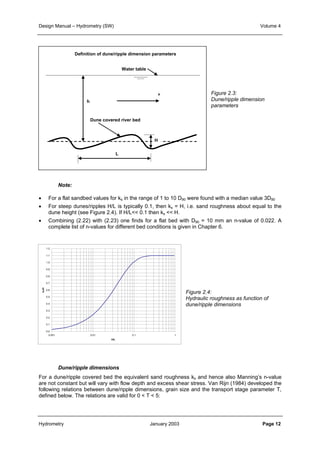
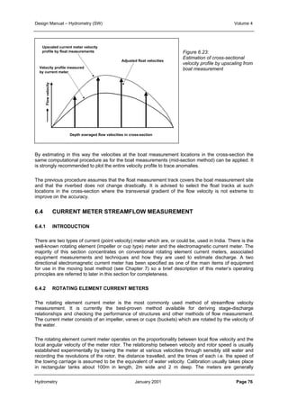
Some practical relations for ks
According to van Rijn (1984) for an alluvial bed the following values apply for the equivalent sand
roughness ks:
• For a flat sandbed and gravelbed it follows respectively:
k 3D (sandbed) k D (gravelbed) s 90 s 90 ≈ ≈
• For a dune/ripple covered bed (see Figure 2.3)
H
))
L
k 1.1H(1 exp( 25 s ≈ − −
(2.21)
(2.22)
(2.23)
(2.24)
where: D90 = characteristic grain size diameter (90% is finer)
H = dune/ripple height
L = dune/ripple length
H/L = dune/ripple steepness
Hydrometry January 2003 Page 11](https://image.slidesharecdn.com/swvolume4designmanualhydrometry-140924050537-phpapp02/85/Hydrometry-Design-Manual-Volume-4-2003-15-320.jpg)
![Design Manual – Hydrometry (SW) Volume 4
For more accurate computations one can apply the Bresse function. For a wide river the set of
equations to solve read (Chow, 1959):
[ { }]
γ = −
( ) ( ) ( )
x 0 x 0
; 1 Fr
η +
h
n
= − η − η − γ ψ η − ψ η
η =
−
0
L
x
where :
S
Δ +
h h
x n
n
;
2
η + η +
η −
η =
x
and
ψ η =
Δ +
2 1
3
h h
1
0 n
h
n
arc cot g
3
( 1)
1
1
h
ln
6
( )
2
2
(2.46)
The function Ψ(η) for 1 ≤ η < 1.25 is presented in Table 2.3. An application is presented in Example
2.1.
η Ψ η Ψ η Ψ η Ψ η Ψ
1.000 ∞ 1.050 0.896 1.100 0.681 1.150 0.561 1.200 0.480
1.001 2.184 1.051 0.889 1.101 0.678 1.151 0.559 1.201 0.478
1.002 1.953 1.052 0.883 1.102 0.675 1.152 0.557 1.202 0.477
1.003 1.818 1.053 0.877 1.103 0.672 1.153 0.555 1.203 0.476
1.004 1.723 1.054 0.871 1.104 0.669 1.154 0.553 1.204 0.474
1.005 1.649 1.055 0.866 1.105 0.666 1.155 0.551 1.205 0.473
1.006 1.588 1.056 0.860 1.106 0.663 1.156 0.550 1.206 0.472
1.007 1.537 1.057 0.854 1.107 0.660 1.157 0.548 1.207 0.470
1.008 1.493 1.058 0.849 1.108 0.657 1.158 0.546 1.208 0.469
1.009 1.454 1.059 0.843 1.109 0.655 1.159 0.544 1.209 0.468
1.010 1.419 1.060 0.838 1.110 0.652 1.160 0.542 1.210 0.466
1.011 1.388 1.061 0.833 1.111 0.649 1.161 0.541 1.211 0.465
1.012 1.359 1.062 0.828 1.112 0.647 1.162 0.539 1.212 0.464
1.013 1.333 1.063 0.823 1.113 0.644 1.163 0.537 1.213 0.463
1.014 1.308 1.064 0.818 1.114 0.641 1.164 0.535 1.214 0.461
1.015 1.286 1.065 0.813 1.115 0.639 1.165 0.534 1.215 0.460
1.016 1.264 1.066 0.808 1.116 0.636 1.166 0.532 1.216 0.459
1.017 1.245 1.067 0.804 1.117 0.634 1.167 0.530 1.217 0.458
1.018 1.226 1.068 0.799 1.118 0.631 1.168 0.528 1.218 0.456
1.019 1.208 1.069 0.795 1.119 0.628 1.169 0.527 1.219 0.455
1.020 1.191 1.070 0.790 1.120 0.626 1.170 0.525 1.220 0.454
1.021 1.175 1.071 0.786 1.121 0.624 1.171 0.523 1.221 0.453
1.022 1.160 1.072 0.781 1.122 0.621 1.172 0.522 1.222 0.451
1.023 1.146 1.073 0.777 1.123 0.619 1.173 0.520 1.223 0.450
1.024 1.132 1.074 0.773 1.124 0.616 1.174 0.519 1.224 0.449
1.025 1.119 1.075 0.769 1.125 0.614 1.175 0.517 1.225 0.448
1.026 1.106 1.076 0.765 1.126 0.612 1.176 0.515 1.226 0.447
1.027 1.094 1.077 0.760 1.127 0.609 1.177 0.514 1.227 0.445
1.028 1.082 1.078 0.756 1.128 0.607 1.178 0.512 1.228 0.444
1.029 1.071 1.079 0.753 1.129 0.605 1.179 0.511 1.229 0.443
1.030 1.060 1.080 0.749 1.130 0.602 1.180 0.509 1.230 0.442
1.031 1.049 1.081 0.745 1.131 0.600 1.181 0.507 1.231 0.441
1.032 1.039 1.082 0.741 1.132 0.598 1.182 0.506 1.232 0.440
1.033 1.029 1.083 0.737 1.133 0.596 1.183 0.504 1.233 0.438
1.034 1.019 1.084 0.734 1.134 0.594 1.184 0.503 1.234 0.437
1.035 1.010 1.085 0.730 1.135 0.591 1.185 0.501 1.235 0.436
1.036 1.001 1.086 0.726 1.136 0.589 1.186 0.500 1.236 0.435
1.037 0.992 1.087 0.723 1.137 0.587 1.187 0.498 1.237 0.434
1.038 0.983 1.088 0.719 1.138 0.585 1.188 0.497 1.238 0.433
1.039 0.975 1.089 0.716 1.139 0.583 1.189 0.495 1.239 0.432
1.040 0.967 1.090 0.713 1.140 0.581 1.190 0.494 1.240 0.431
1.041 0.959 1.091 0.709 1.141 0.579 1.191 0.492 1.241 0.429
1.042 0.951 1.092 0.706 1.142 0.577 1.192 0.491 1.242 0.428
1.043 0.944 1.093 0.703 1.143 0.575 1.193 0.490 1.243 0.427
1.044 0.936 1.094 0.699 1.144 0.573 1.194 0.488 1.244 0.426
1.045 0.929 1.095 0.696 1.145 0.571 1.195 0.487 1.245 0.425
1.046 0.922 1.096 0.693 1.146 0.569 1.196 0.485 1.246 0.424
1.047 0.915 1.097 0.690 1.147 0.567 1.197 0.484 1.247 0.423
1.048 0.909 1.098 0.687 1.148 0.565 1.198 0.483 1.248 0.422
1.049 0.902 1.099 0.684 1.149 0.563 1.199 0.481 1.249 0.421
Table 2.3: The function Ψ(η) for 1 ≤ η < 1.25
Hydrometry January 2003 Page 19](https://image.slidesharecdn.com/swvolume4designmanualhydrometry-140924050537-phpapp02/85/Hydrometry-Design-Manual-Volume-4-2003-23-320.jpg)
![Design Manual – Hydrometry (SW) Volume 4
Example 2.1 Application of Bresse function
The distance is to be determined over which the backwater effect at x = 0 of 1 m is reduced to 5% of its
original value for a river with a bed slope of 5x10⁻⁴, hydraulic roughness n = 0.03, when the normal depth hn
= 5 m.
1. Determination of η and Ψ(η)
For x = 0 the backwater is Δh0 = 1m hence η0 becomes:
1.20
+
1.0 5.0
Δ +
η =
0 =
5.0
h h
0 n
h
n
=
If x = x1 is the distance at which the initial backwater effect is reduced to 5% of its value: Δh1 = 0.05 m,
hence η1 becomes:
1.01
+
0.05 5.0
Δ +
η =
1 =
5.0
h h
1 n
h
n
=
It then follows for Ψ(η0) and Ψ(η1) from Table 2.3: Ψ(η0) = 0.480 and Ψ(η1) = 1.419
2. Froude correction γ:
−
1/3 4
5 x5x10
γ 2 = − = − = − =
9.81x0.03
1
1/3
n
h S
gn
1
v
2
gh
= 1- Fr 1
2
2
0
The parameter γ in equation (2.46) follows from:
3. Computation of Lx
0.903
The distance Lx = x1 – x0 follows from (2.46) by substitution of the values determined under 1 and 2:
h
h
[ { }] [ ] n
10,380m 10.4km
x = − η − η − γ Ψ η − Ψ η = − − − − = = =
S
(1.01 1.2) 0.903x(1.419 0.480) 1.038x
n
S
( ) ( ) ( )
h
n
S
L
0
0
1 0 1 0
0
Note that the distance is only 4% larger than one would have obtained from (2.45). The results (Lx at 5% of
the original value, expressed as a function of hn/S0) for different river slopes and roughness values for the
same normal depth (5 m) and initial backwater (1 m) are presented in the following table:
Froude parameter γ Lx expressed as function of hn/S0
Roughness n Roughness n
S0
0.025 0.03 0.05 0.025 0.03 0.05
1x10⁻³
5x10⁻⁴
1x10⁻⁴
0.721
0.861
0.972
0.806
0.903
0.981
0.930
0.965
0.993
0.867
0.998
1.103
0.947
1.038
1.111
1.063
1.096
1.122
It is observed, that the multiplier to hn/S0, to arrive at Lx , is close to 1 for different river slopes and
roughness values. Adding some 10% to the value for Lx obtained from (2.45) will give a reasonable
approximation of the extent of the backwater reach in practice for field applications.
Hydrometry January 2003 Page 20](https://image.slidesharecdn.com/swvolume4designmanualhydrometry-140924050537-phpapp02/85/Hydrometry-Design-Manual-Volume-4-2003-24-320.jpg)
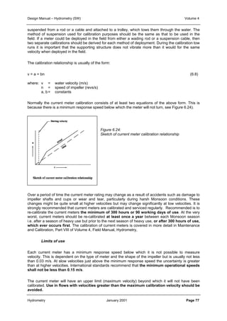
![Design Manual – Hydrometry (SW) Volume 4
manner in which the rating tank conditions resemble reality (being towed in stagnant water or being
kept steady in a turbulent flow is not the same!!)
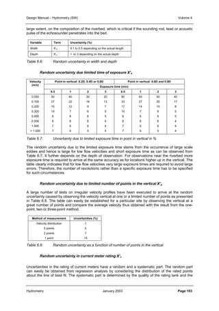
The random error part in the current meter rating is presented in Table 6.9. The data is based on
experiments performed in several rating tanks. A distinction is made between individual rating and
group rating.
Velocity (m/s) Uncertainties (%)
Individual rating Group or standard
rating
0.03
0.10
0.15
0.25
0.50
0.50
20
5
2.5
2
1
1
20
10
5
4
3
2
Table 6.9:
Random uncertainty in current meter
rating, X’c
Systematic uncertainty in width X”b, depth X”d and current meter rating X”c
Variable Term Uncertainty (%)
Width
Depth
Current meter rating
X”b
X”d
X”c
0.5
0.5
1.0
Table 6.10: Systematic uncertainty in width X”b, depth X”d and current meter rating X”c
Typical order of magnitude values for systematic uncertainties in the measurement of the width and
depth and in current meter rating caused by the rating tank characteristics and the method of
calibration are presented in Table 6.10.
Application
To illustrate the use of the error analysis a few examples are worked out in the following.
Example 6.3
Conditions: River discharge Q = 120 m3/s
Number of verticals = 20
Average velocity = 0.60 m/s
Method used = 1-point method (0.6D), 60 seconds exposure
Computation of error:
X’n = 5% (Table 6.5)
X’b = 0.3% (Table 6.6)
X’d = 2% (Table 6.6)
X’e = 6% (Table 6.7)
X’p = 15% (Table 6.8)
X’c = 1% (Table 6.9, individual rating)
X”b = 0.5% (Table 6.10)
X”d = 0.5% (Table 6.10)
X”c = 1% (Table 6.10)
With (6.14) the random error becomes:
X’Q = [52 + 1/20(0.32 +22 + 62 + 152 + 12)]1/2 =[25 + 266/20]1/2 = 6.2%
From (6.15) the systematic error amounts:
X”Q = [0.52 + 0.52 + 12]1/2 = 1.2%
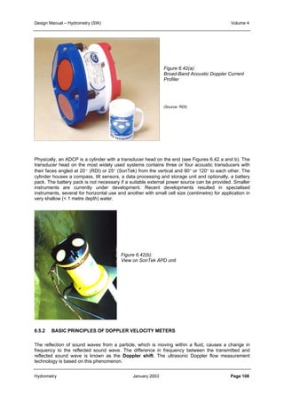
Hydrometry January 2003 Page 104](https://image.slidesharecdn.com/swvolume4designmanualhydrometry-140924050537-phpapp02/85/Hydrometry-Design-Manual-Volume-4-2003-108-320.jpg)
![Design Manual – Hydrometry (SW) Volume 4
Finally, using (6.16) the overall uncertainty in the discharge becomes:
XQ = [6.2 2 + 1.2 2]1/2 = 6.3%
Hence the discharge is Q = 120 m3/s ± 6.3%
In official documents according to ISO standards random and systematic uncertainties have to be specified
separately; so the statement becomes:
Discharge = 120 m3/s ± 6.3%, random uncertainty = ± 6.2%, systematic uncertainty =± 1.2%
Note that the true discharge is likely to lie between 112.4 and 127.6 m3/s, Hence there are 3 significant
digits. So it makes no sense to present the discharge in this case with 1 or more decimals, see also
Volume 2, Design Manual, Sampling Principles.
Example 6.4
Conditions: similar to EXAMPLE 6.3 but instead of using a 1-point method, the 0.2D0.8D, i.e the
2-point method is used in the verticals.
It is easily observed that the use of the 2-point method only changes the uncertainty due to the number of
points in the vertical X’p. For the 2-point method one gets from Table 6.8: X’p = 7%. The random
uncertainty then becomes
X’Q = [52 + 1/20(0.32 +22 + 62 + 72 + 12)]1/2 =[25 + 90/20]1/2 = 5.4%, instead of 6.2% for the 1-point method.
The overall uncertainty now reads: XQ = [5.42 + 1.22]1/2 = 5.5%, which is only a marginal improvement
compared to the 6.3% before.
Example 6.5
Conditions: similar to EXAMPLE 6.3, but the velocity is now observed at 10 verticals only.
The change in the number of verticals affects only the random part of the uncertainty. From (6.14) and
Table 6.5 one obtains for X’n = 9%. The other effect of this change is that the denominator (n) in (6.14) also
changes. The random uncertainty then becomes
X’Q = [92 + 1/10(0.32 +22 + 62 + 152 + 12)]1/2 =[81 + 266/10]1/2 = 10.4%, instead of 6.2% for sampling at 20
verticals.
The overall uncertainty now reads: XQ = [10.42 + 1.22]1/2 = 10.5%, which is considerably worse than in the
two examples before.
The results from the examples are summarised and extended in Table 6.11.
Random uncertainty in discharge
X’Q
Overall uncertainty in discharge
XQ
Number of verticals
1-point 2-points 1-point 2-points
10 10.4 9.5 10.5 9.6
20 6.2 5.4 6.3 5.6
30 4.2 3.5 4.4 3.7
40 2.6 2.5 2.9 2.8
Table 6.11: Effect of number of verticals and number of points in the vertical on uncertainty in Q
From the theory and the examples it follows that:
• The most important factor to keep the uncertainty in Q low is to measure the velocity in a
sufficient number of verticals (≥ 20)
• The reduction in the uncertainty in Q from measuring at two points rather than in one point is
marginal.
Hydrometry January 2003 Page 105](https://image.slidesharecdn.com/swvolume4designmanualhydrometry-140924050537-phpapp02/85/Hydrometry-Design-Manual-Volume-4-2003-109-320.jpg)