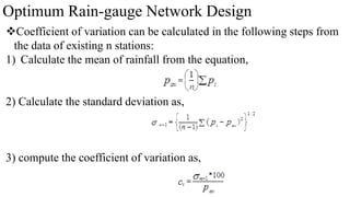
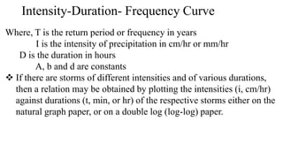
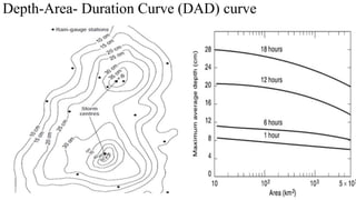
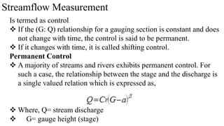
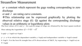
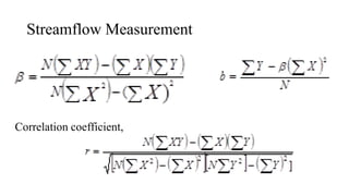
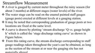
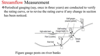
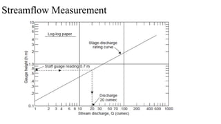
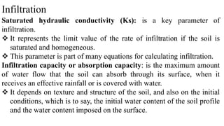
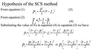
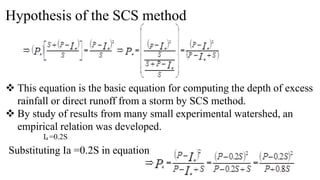
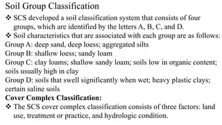
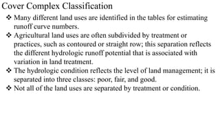
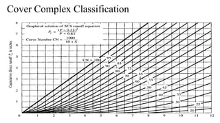
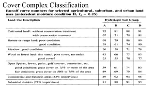
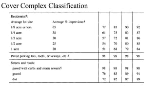
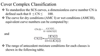
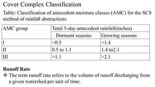
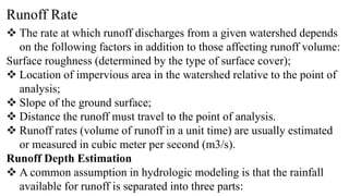
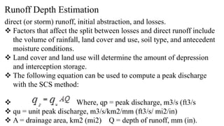
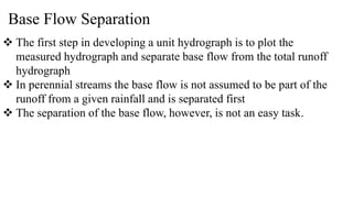
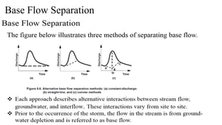
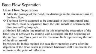
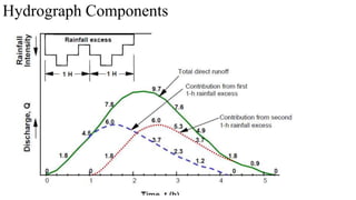
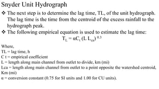
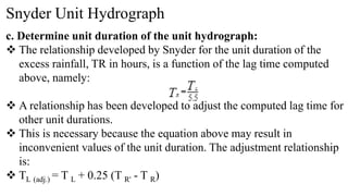
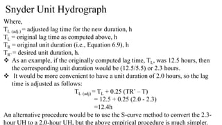
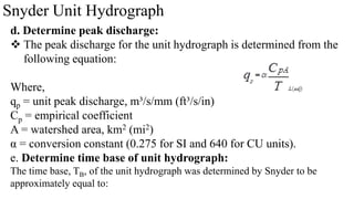
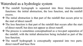
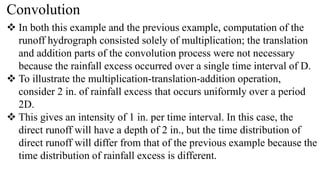
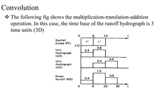
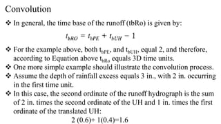
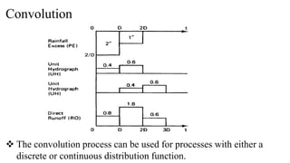
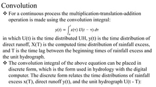
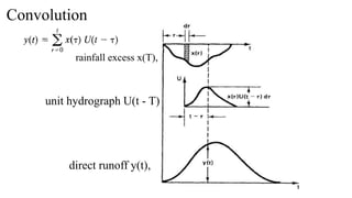
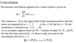
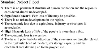
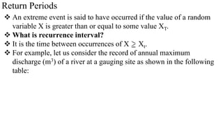
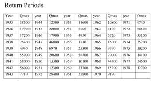
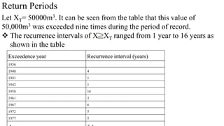
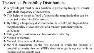
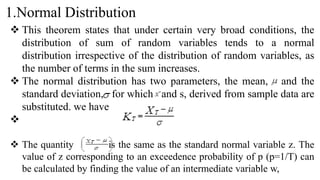
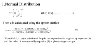
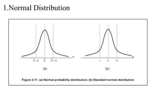
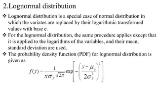
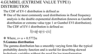
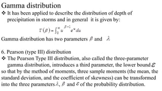
This document provides an overview of the course "Applied Hydrology" at Wollega University. The course is part of the Master of Science program in Hydraulic Engineering. It covers key topics in hydrology including the hydrologic cycle, hydrologic abstractions, infiltration, evaporation, and hydrologic measurements. Engineering applications of hydrology principles are also discussed such as design of irrigation systems, dams, and flood control projects.

![Hydro-meteorological measurement and data analysis
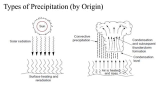
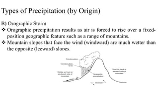
The formation of precipitation requires a four step process:
(1) Cooling of air to approximately the dew-point temperature;
(2) Condensation on nuclei to form cloud droplets or ice crystals;
(3) Growth of droplets or crystals into rain drops, snowflakes or
hailstones and
(4) Importation of water vapor to sustain the process of precipitation
geographically, temporally, and seasonally.
This regional and temporal variation in precipitation are important in
water resources planning and hydrologic studies.
The amount fallen is usually expressed in terms of precipitation depth
per unit of horizontal area [mm] or in terms of intensity[mm/h], which](https://image.slidesharecdn.com/appliedhydrology-230811074648-e5ff0e9a/85/Applied-Hydrology-pptx-35-320.jpg)

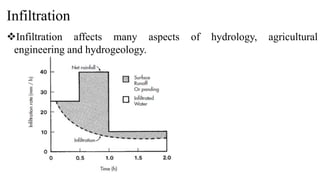
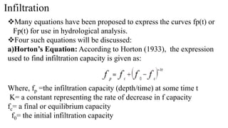
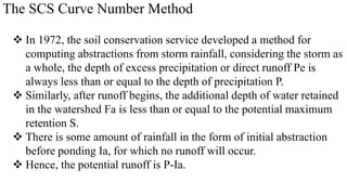
![Infiltration
Where, I(t) is the cumulative infiltration at time t [mm] and i(t) is the
rate of infiltration for time t [mm/h].
Figure General Evolution of the rate of infiltration and of cumulative
infiltration over time (Ks = saturated hydraulic conductivity)](https://image.slidesharecdn.com/appliedhydrology-230811074648-e5ff0e9a/85/Applied-Hydrology-pptx-136-320.jpg)
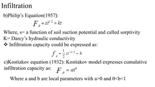
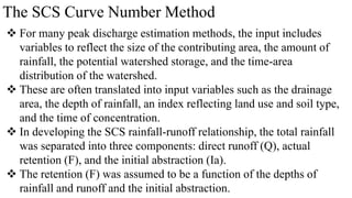
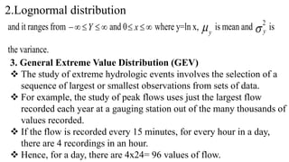
![3. General Extreme Value Distribution (GEV)
The parameters α and u are estimated by
∝=
U=
The parameter u is the mode of the distribution (point of maximum
probability density). A reduced variate y can be defined as:
Substituting the reduced variate in the above equation gives:
F(x) =exp [-exp {-y}]](https://image.slidesharecdn.com/appliedhydrology-230811074648-e5ff0e9a/85/Applied-Hydrology-pptx-307-320.jpg)
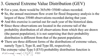
![3. General Extreme Value Distribution (GEV)
Taking ln on either sides of equation we have,
ln F(x)= ln[exp{-exp(-y)}]=-exp(-y)=-1/ex=ey=
Taking ln on both sides of the above equation, we have,
ln (ey)=-ln
This equation is used to define y for the type II and type III
distributions.
For the extreme value type I (EVI) distributions, the plot is a straight
line.
For large values of y, the corresponding curve for the extreme value type
II (EVII) distribution slopes more steeply than for EVI, and the curve for
the EVIII distribution slopes less steeply, being bounded from above.](https://image.slidesharecdn.com/appliedhydrology-230811074648-e5ff0e9a/85/Applied-Hydrology-pptx-308-320.jpg)
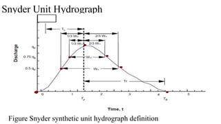
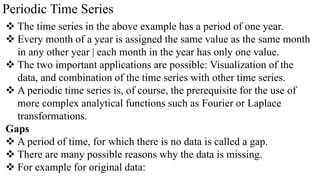
![Time Intervals
A time interval is an interval in the mathematical sense, and a subset
of the set time.
An interval is specified by a starting point ‘a’ and end point ‘b’, and is
an interval of the form (a; b].
Periods of Time
A period of time is either the length of an interval of time or a length
of time designated by such terms as Month", or year".
These do not have identical lengths, but are nonetheless similar to one
another.
Multiples of periods of time are allowed in addition to the basic unit.
Types of Time Series
Every quality of a time series has a value function associated with it.](https://image.slidesharecdn.com/appliedhydrology-230811074648-e5ff0e9a/85/Applied-Hydrology-pptx-320-320.jpg)
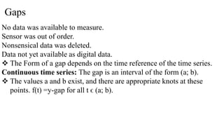
![Continuous time series:
Interval time series: The gap is a time interval, which thus has the
form (a; b].
Fig. Gaps in an interval time series
Fig. Gaps in a continuous time series](https://image.slidesharecdn.com/appliedhydrology-230811074648-e5ff0e9a/85/Applied-Hydrology-pptx-330-320.jpg)
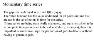
![Momentary time series
N.B. Equidistant interval time series do not necessarily have gaps which
are the length of an interval; a gap could also be some multiple of this
interval. f(t) = y-gap for all t ϵ (a; b]
Momentary time series: A gap in a momentary time series is a single
point in time.](https://image.slidesharecdn.com/appliedhydrology-230811074648-e5ff0e9a/85/Applied-Hydrology-pptx-331-320.jpg)


![Civil v-hydrology and irrigation engineering [10 cv55]-notes](https://cdn.slidesharecdn.com/ss_thumbnails/civil-v-hydrologyandirrigationengineering10cv55-notes-160425135643-thumbnail.jpg?width=640&height=640&fit=bounds)


