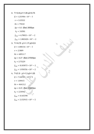
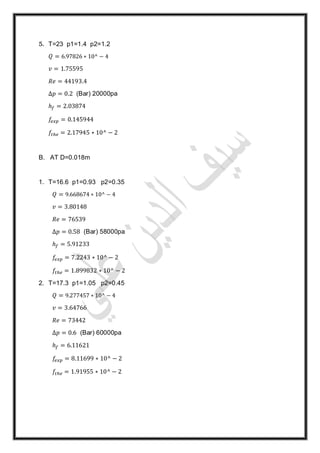
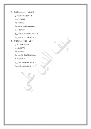
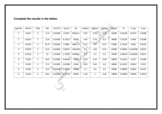
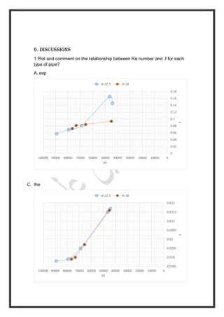
The document outlines an experiment conducted at Baghdad University to measure friction loss along pipes of various diameters and flow rates, aiming to compare experimental results of the Darcy-Weisbach coefficient with theoretical values. It details the apparatus used, theoretical background on pressure loss and friction factor calculations, and a step-by-step experimental procedure. Results and discussions explore the relationship between Reynolds number and friction factor, as well as the impact of diameter changes on head loss.

1. Baghdad University
College of Engineering
Department of Mechanical Engineering
Name of Experiment
'Friction loss along a pipe'
Preparation;
Saif al-Din Ali Madi
the second phase
Group "A"

2. 1. Experiment name: friction loss along a pipe
2. Objective
The objective of this experiment is to measure the head loss in pipes of
different diameters and at different flow rates, as well as to compute
experimental values of the Darcy-Welsbach coefficient (friction factor) f, and
then compare them with theoretical value
3. Apparatus
Apparatus for fluid flow friction in pipes as shown in Fig. 1,
1. The pipe flow rig with pipes of different diameters
D1 = 22.5 mm (smooth pipe)
D2 =18 mm (rough pipe)
D3 =17.8 mm (smooth pipe)
2. Tank used to measure the volume of water flowing out of the system
3. A stop watch used to measure the time required to collect the water
4. A pump for refilling the water reservoir

3. 4. Theory
Losses in pipe networks could be divided typically into major and minor
losses: Major Losses are produced mainly due to friction or viscous action
while miner losses are due to valves bends, elbows, sudden expansion or
contraction, etc.
Experimental
Friction losses in pipes are estimated by Darcy-Welsbach formula as:
Energy equation:-
𝑝1
𝑦
+
𝑣1
2
2𝑔
+ 𝑧1 =
𝑝2
𝑦
+
𝑣2
2
2𝑔
+ 𝑧2 + ℎ𝑓
V1=V2 constant cross sectional area
Z1=Z2 the pipe line at the same level
So:
ℎ𝑓 =
𝑝1
𝑦
−
𝑝2
𝑦
=
𝑝1−𝑝2
𝑦
Or:
∆ℎ =
∆𝑝
𝑦
Pressure loss
The pressure loss (or major loss) in a pipe, tube or duct can be calculated
with the Darcy-Welsbach equation
∆𝑝 = 𝑓
𝐿
𝐷
𝜌𝑣2
2
Head Loss
Alternately, the Darcy-Welsbach equation (3) can also express the head loss
as
ℎ𝑓 = 𝑓
𝐿
𝐷
𝑣2
2𝑔

4. Where
∆𝑝 - Pressure loss (Pa, N / 𝑚2
)
ℎ𝑓 -Head loss due to friction (m)
L - Is the length of the pipe (m)
D is the diameter of the pipe (m)
V- Is the average velocity of the fluid flow (m /s)
g- Is the acceleration due to gravity (m /𝑠2)
f- Is a dimensionless coefficient called the Darcy friction factor.
Calculate velocity of the fluid flow
𝑄 =
𝑉
𝑡
𝑉 =
4𝑄
𝜋𝐷2
Where;
V =Volume of water, 𝑚3
(V=A*B) (3.5 cm, B-15 cm, c=20cm)
Q=volumetric flow rate (𝑚3/ s) 20 cm)
Theoretical
Friction coefficient "f" is a function of Reynolds number and inner surface
roughness of the pipe. In the Laminar flow (Re ≤ 2000) it was calculated to be;
fth =
64
Re
(Hagen-Poiseuille equation)
While for Large value of Re (10 * <Re <10) Blasius found it to be as:
fth =
0.316
Re0.25
(Blasius equation)

5. Calculate Re number:
𝑅𝑒 =
𝜌𝑣𝐷
𝜇
Where:
𝜌 = 1000 𝑘𝑔/𝑚3
𝜇 = 0.894 × 10−3
𝑚2
/𝑠
∀= 𝐴 ∗ 𝐵 ∗ 𝐶
𝑄 = ∀/𝑡
𝑣 = 4𝑄/𝜋𝑑2
𝑅𝑒 =
𝜌𝑣𝐷
𝜇
∆𝑝 = 𝑝1 − 𝑝2 (Bar)
ℎ𝑓 = ∆𝑝(𝑝𝑎)/𝛾
𝑓𝑒𝑥𝑝 = 2ℎ 𝑓 𝐷𝑔/𝐿𝑣2
𝑓𝑡ℎ𝑒 = 0.316/Re0.25
4. Experimental procedure
1. Open the valves across she pipe along which the friction los will pe along
which the friction loss will be calculated, and ensure that all the other valves
for the other pipes are closed.
2. Record the readings on the pressures p1 and p2
3. The water tank was emptied of water and the refilled to take reading of time
versus volume which was used to calculate the volumetric rate of flow.
4. Repeat the above procedure for a new value of flow rates. This could be
ensured by adjusting the closure of the gate valve in equally spaced over the
full flow range.
5. Repeat the above procedure for a new pipe.

6. 5. Results and calculations
𝜌=1000 𝜇 =0.894*0.001 𝛾 =9810 L=2
A. At D=0.0225 m
∀= 20 ∗ 15 ∗ 53.5 = 0.01605
1. T=11.4 p1=0.87 p2=0.55
Q=V/t
Q= 0.01605/11.4=1.407*10^-3
𝑣 = 4𝑄/𝜋𝑑2
V=4*1.407*10^-3 / 3.41*0.0225^2=3.5427
𝑅𝑒 =
𝜌𝑣𝐷
𝜇
Re=1000*3.5427*0.0225 / 0.894*0.001 =89162.1
∆𝑝 = 𝑝1 − 𝑝2 (Bar)
∆𝑝 = 0.87 − 0.55 = 0.32 𝑏𝑎𝑟 = 32000𝑝𝑎
ℎ𝑓 = ∆𝑝(𝑝𝑎)/𝛾
ℎ𝑓 = 32000/9810 =3.26189
𝑓𝑒𝑥𝑝 = 2ℎ 𝑓 𝐷𝑔/𝐿𝑣2
𝑓𝑒𝑥𝑝=2*3.26189*0.0225*9.81 / 2*3.43271^2 = 5.736693*10^-2
𝑓𝑡ℎ𝑒 = 0.316/Re0.25
𝑓𝑡ℎ𝑒=0.316 / 89162.1^2 = 1.828698*10^-2

7. 2. T=12.8 p1=1.05 p2=0.75
𝑄 = 1.253906 ∗ 10^ − 3
𝑣 = 3.15522
𝑅𝑒 = 79410
∆𝑝 = 0.3 (Bar) 3000pa
ℎ𝑓 = 3.0581
𝑓𝑒𝑥𝑝 = 6.78021 ∗ 10^ − 2
𝑓𝑡ℎ𝑒 = 1.882428 ∗ 10^ − 2
3. T=14.75 p1=1.17 p2=0.9
𝑄 = 1.088136 ∗ 10^ − 3
𝑣 = 2.3809
𝑅𝑒 = 68911.7
∆𝑝 = 0.27 (Bar) 27000pa
ℎ𝑓 = 2.75229
𝑓𝑒𝑥𝑝 = 8.103073 ∗ 10^ − 2
𝑓𝑡ℎ𝑒 = 1.950356 ∗ 10^ − 2
4. T=21.9 p1=1.3 p2=1.05
𝑄 = 7.328767 ∗ 10^ − 4
𝑣 = 1.84415
𝑅𝑒 = 46413.2
∆𝑝 = 0.25 (Bar) 25000pa
ℎ𝑓 = 2.54942
𝑓𝑒𝑥𝑝 = 0.165398
𝑓𝑡ℎ𝑒 = 2.152915 ∗ 10^ − 2

8. 5. T=23 p1=1.4 p2=1.2
𝑄 = 6.97826 ∗ 10^ − 4
𝑣 = 1.75595
𝑅𝑒 = 44193.4
∆𝑝 = 0.2 (Bar) 20000pa
ℎ𝑓 = 2.03874
𝑓𝑒𝑥𝑝 = 0.145944
𝑓𝑡ℎ𝑒 = 2.17945 ∗ 10^ − 2
B. AT D=0.018m
1. T=16.6 p1=0.93 p2=0.35
𝑄 = 9.668674 ∗ 10^ − 4
𝑣 = 3.80148
𝑅𝑒 = 76539
∆𝑝 = 0.58 (Bar) 58000pa
ℎ𝑓 = 5.91233
𝑓𝑒𝑥𝑝 = 7.2243 ∗ 10^ − 2
𝑓𝑡ℎ𝑒 = 1.899832 ∗ 10^ − 2
2. T=17.3 p1=1.05 p2=0.45
𝑄 = 9.277457 ∗ 10^ − 4
𝑣 = 3.64766
𝑅𝑒 = 73442
∆𝑝 = 0.6 (Bar) 60000pa
ℎ𝑓 = 6.11621
𝑓𝑒𝑥𝑝 = 8.11699 ∗ 10^ − 2
𝑓𝑡ℎ𝑒 = 1.91955 ∗ 10^ − 2

9. 3. T=19.3 p1=1.1 p2=0.6
𝑄 = 8.31606 ∗ 10^ − 4
𝑣 = 3.26966
𝑅𝑒 = 65832
∆𝑝 = 0.5 (Bar) 50000pa
ℎ𝑓 = 5.09684
𝑓𝑒𝑥𝑝 = 8.41853329 ∗ 10^ − 2
𝑓𝑡ℎ𝑒 = 1.972775 ∗ 10^ − 2
4. T=28.2 p1=1.26 p2=1
𝑄 = 5.65 ∗ 10^ − 4
𝑣 = 2.23775
𝑅𝑒 = 45055
∆𝑝 = 0.26 (Bar) 26000pa
ℎ𝑓 = 2.65036
𝑓𝑒𝑥𝑝 = 9.345948 ∗ 10^ − 2
𝑓𝑡ℎ𝑒 = 2.168955 ∗ 10^ − 2

10. Complete the results in the tables:
pipe No. D(mm) L(M) t(S) V(m^3) v(m/s) Re p1(bar) p2(bar) ∆p(bar) ∆p(pa) hf f_exp f_the
1 0.023 2 11.4 0.01605 3.5427 89162.1 0.87 0.55 0.32 32000 3.26189 0.0573 0.0188
2 0.0225 2 12.8 0.01605 3.15522 79410 1.05 0.75 0.3 30000 2.75229 0.069 0.0189
3 0.0225 2 14.75 0.01605 2.3809 68911.7 1.17 0.9 0.27 27000 2.75229 0.081 0.0195
4 0.0225 2 21.9 0.01605 1.84415 46413.2 1.3 1.05 0.25 25000 2.54942 0.165398 0.0215
5 0.0225 2 23 0.01605 1.75595 44193.4 1.4 1.2 0.2 20000 2.03874 0.145944 0.0217
6 0.018 2 16.6 0.01605 3.80148 76539 0.93 0.35 0.58 58000 5.91233 0.072 0.0189
7 0.018 2 17.3 0.01605 3.64766 73442 1.05 0.45 0.6 60000 6.11621 0.0811 0.019
8 0.018 2 19.3 0.01605 3.26966 65832 1.1 0.6 0.5 50000 5.09684 0.0841 0.0197
9 0.018 2 28.2 0.01605 2.23775 45055 1.26 1 0.26 26000 2.65036 0.0934 0.0216

11. 6. Discussions
1 Plot and comment on the relationship between Re number and .f for each
type of pipe?
A. exp
C. the
0
0.02
0.04
0.06
0.08
0.1
0.12
0.14
0.16
0.18
0100002000030000400005000060000700008000090000100000
F
RE
d=22.5 d=18
0.0185
0.019
0.0195
0.02
0.0205
0.021
0.0215
0.022
0100002000030000400005000060000700008000090000100000
F
RE
d=22.5 d=18

12. 2. What is the effect of changing the value of the diameter or on hf?
The inverse relationship between the hf and the diameter of any increase
occurs to the diameter of the reduction of the value of hf according to the
following law
ℎ𝑓 = 𝑓
𝐿
𝐷
𝑣2
2𝑔
3. What is the effect of changing the water to oil or engine oil on hf?
Viscosity of oil great than viscosity of water
ᵔ Viscosity of oil > viscosity of water
ᵕ Re oil < Re water
𝑅𝑒 =
𝜌𝑣𝐷
𝜇
Inverse relationship
ᵔ Re oil < Re water
F oil > f water
4. What suggestion have you to improving the apparatus?
1. Pressure control by accurate sensors that take readings
2. Develop the reservoir so that the accurate sampling and connection with the
sensor to take the exact time
3. His reading scale put the amount of flow to compare
4. Taking into account the safety and handling of electricity system development
of the control of the protection of the