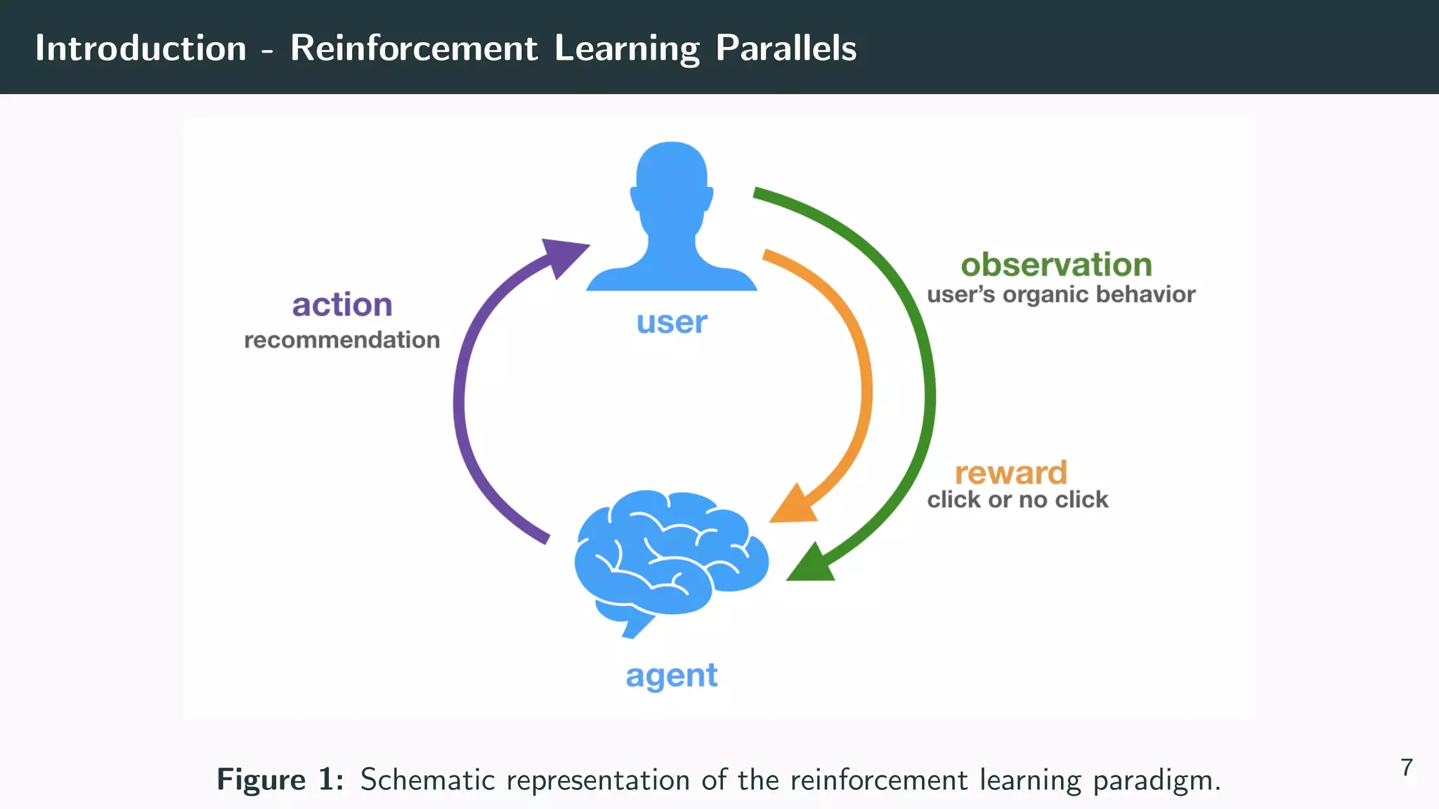
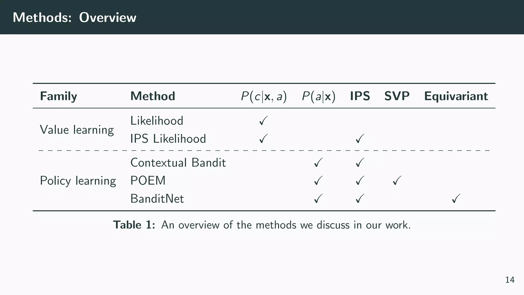
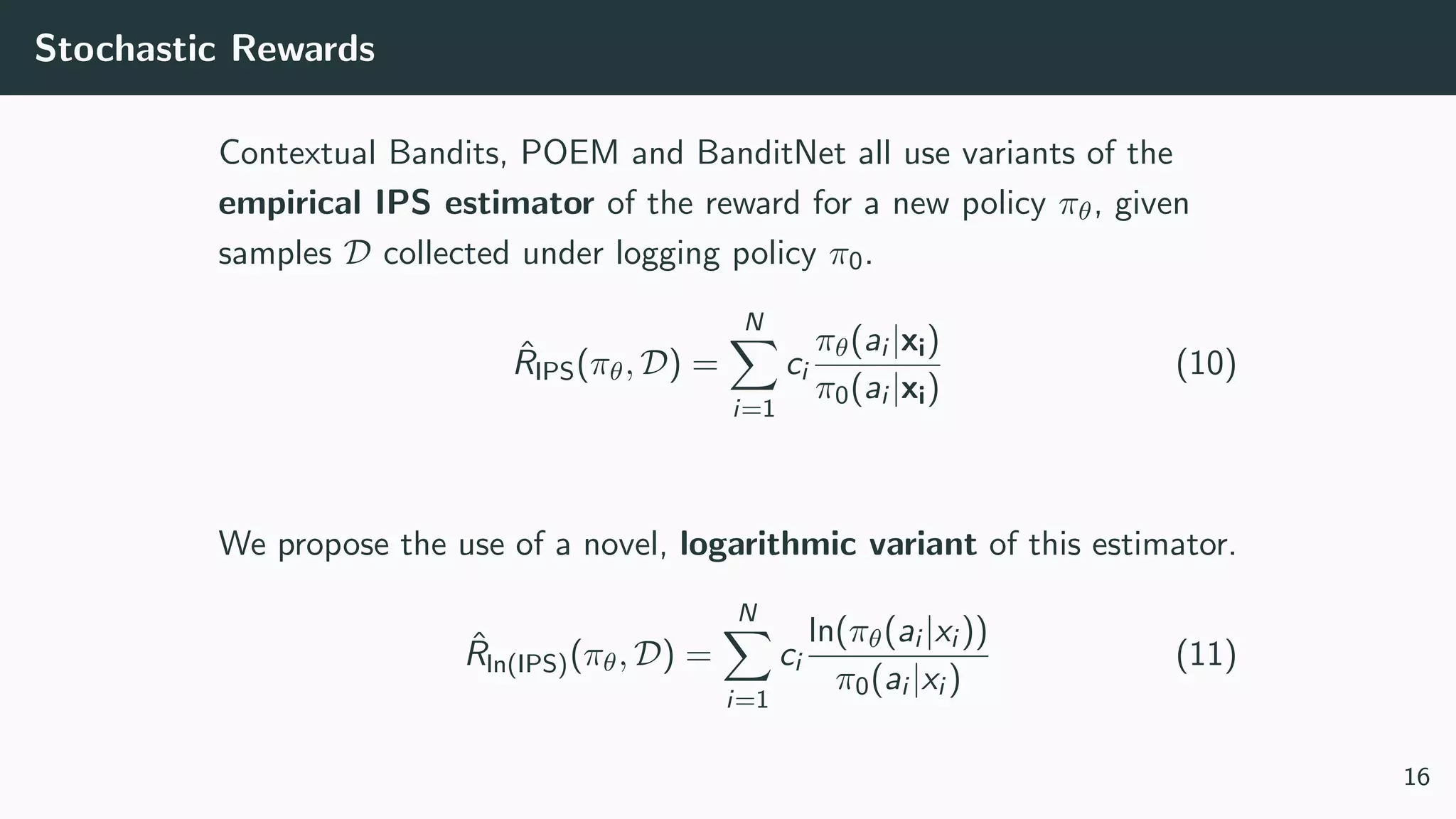
Counterfactual Learning for Recommendation
Olivier Jeunen,
Dmytro Mykhaylov, David Rohde, Flavian Vasile, Alexandre Gilotte, Martin Bompaire
September 25, 2019
Adrem Data Lab, University of Antwerp
Criteo AI Lab, Paris
olivier.jeunen@uantwerp.be
1
Table of contents
1. Introduction
2. Methods
3. Learning for Recommendation
4. Experiments
5. Conclusion
2
Introduction
Introduction - Recommender Systems
Motivation
• Web-scale systems (Amazon, Google, Netflix, Spotify,. . . )
typically have millions of items in their catalogue.
• Users are often only interested in a handful of them.
• Recommendation Systems aim to identify these items for every user,
encouraging users to engage with relevant content.
3
4
Introduction
Traditional Approaches
• Typically based on collaborative
filtering on the user-item matrix:
o Nearest-neighbour models,
o Latent factor models,
o Neural networks,
o . . .
• Goal is to identify which items the user
interacted with in a historical dataset,
regardless of the recommender.




















0 0 0 . . . 0 1 0
1 0 0 . . . 0 0 1
0 0 0 . . . 1 0 0
0 0 1 . . . 0 0 0
. . . . . . . . . . . . . . . . . . . . .
0 1 0 . . . 0 1 0
0 0 0 . . . 0 1 0
0 1 1 . . . 0 0 0
0 0 0 . . . 1 0 0
1 0 1 . . . 0 1 0




















5
Introduction
Learning from Bandit Feedback
• Why not learn directly from the recommender’s logs?
What was shown in what context and what happened as a result?
• Not straightforward, as we only observe the
result of recommendations we actually show.
• Broad existing literature on Counterfactual Risk Minimisation (CRM)
exists, but has never been validated in a recommendation context.
6
Introduction - Reinforcement Learning Parallels
Figure 1: Schematic representation of the reinforcement learning paradigm. 7
Methods
Background
Notation
We assume:
• A stochastic logging policy π0 that describes a probability distribution
over actions, conditioned on the context.
• Dataset of logged feedback D with N tuples (x, a, p, c) with
x ∈ Rn a context vector (historical counts),
a ∈ [1, n] an action identifier,
p ≡ π0(a|x) the logging propensity,
c ∈ {0, 1} the observed reward (click).
8
Methods: Value-based
Likelihood (Logistic Regression) Hosmer Jr. et al. [2013]
Model the probability of a click, conditioned on the action and context:
P(c = 1|x, a) (1)
You can optimise your favourite classifier for this! (e.g. Logistic Regression)
Obtain a decision rule from:
a∗
= arg max
a
P(c = 1|x, a). (2)
9
Methods: Value-based
IPS-weighted Likelihood Storkey [2009]
Naturally, as the logging policy is trying to achieve some goal (e.g. clicks,
views, dwell time, . . . ), it will take some actions more often than others.
We can use Inverse Propensity Scoring (IPS) to force the error of the fit
to be distributed evenly across the action space.
Reweight samples (x, a) by:
1
π0(a|x)
(3)
10
Methods: Policy-based
Contextual Bandit Bottou et al. [2013]
Model the counterfactual reward:
“How many clicks would a policy πθ have gotten if it was deployed instead of π0?”
Directly optimise πθ, with θ ∈ Rn×n the model parameters:
P(a|x, θ) = πθ(a|x) (4)
θ∗
= arg max
θ
N
i=1
ci
πθ(ai |xi)
π0(ai |xi)
(5)
a∗
= arg max
a
P(a|x, θ) (6)
11
Methods: Policy-based
POEM Swaminathan and Joachims [2015a]
IPS estimators tend to have high variance, clip weights and introduce
sample variance penalisation:
θ∗
= arg max
θ
1
N
N
i=1
ci min M,
πθ(ai |xi)
π0(ai |xi)
− λ
Varθ
N
(7)
12
Methods: Policy-based
NormPOEM Swaminathan and Joachims [2015b]
Variance penalisation is insufficient, use the self-normalised IPS estimator:
θ∗
= arg max
θ
N
i=1 ci
πθ(ai |xi)
π0(ai |xi)
N
i=1
πθ(ai |xi)
π0(ai |xi)
− λ
Varθ
N
(8)
BanditNet Joachims et al. [2018]
Equivalent to a certain optimal translation of the reward:
θ∗
= arg max
θ
N
i=1
(ci − γ)
πθ(ai |xi)
π0(ai |xi)
(9)
13
Methods: Overview
Family Method P(c|x, a) P(a|x) IPS SVP Equivariant
Value learning
Likelihood
IPS Likelihood
Policy learning
Contextual Bandit
POEM
BanditNet
Table 1: An overview of the methods we discuss in our work.
14
Learning for Recommendation
Up until now, most of these methods have been evaluated on a simulated
bandit-feedback setting for multi-class or multi-label classification tasks.
Recommendation, however, brings along specific issues such as:
o Stochastic rewards
o Sparse rewards
15
Stochastic Rewards
Contextual Bandits, POEM and BanditNet all use variants of the
empirical IPS estimator of the reward for a new policy πθ, given
samples D collected under logging policy π0.
ˆRIPS(πθ, D) =
N
i=1
ci
πθ(ai |xi)
π0(ai |xi)
(10)
We propose the use of a novel, logarithmic variant of this estimator.
ˆRln(IPS)(πθ, D) =
N
i=1
ci
ln(πθ(ai |xi ))
π0(ai |xi )
(11)
16
Example: Deterministic Multi-class Rewards
Either action a or b is correct, let’s assume it’s action a.
Thus, we have logged samples (a, c = 1) and (b, c = 0).
0.0 0.2 0.4 0.6 0.8 1.0
p(a) 1 p(b)
0.0
0.5
1.0
1.5
2.0
RIPS
Multi-class rewards
20
15
10
5
0
Rln(IPS)
17
Example: Deterministic Multi-label Rewards
Both action a or b can be correct, let’s assume they are.
Thus, we have logged samples (a, c = 1) and (b, c = 1).
0.0 0.2 0.4 0.6 0.8 1.0
p(a) 1 p(b)
1.90
1.95
2.00
2.05
2.10
RIPS
Multi-label rewards
20
15
10
5
Rln(IPS)
18
Example: Stochastic Multi-label Rewards
Both action a or b can be correct, let’s assume they are. Thus, we can have
logged samples (a, c = 1), (a, c = 0), (b, c = 1) and (b, c = 0).
Assume we have observed 2 clicks on a, and 1 on b.
0.0 0.2 0.4 0.6 0.8 1.0
p(a) 1 p(b)
2.0
2.5
3.0
3.5
4.0RIPS
Stochastic multi-label rewards
20
15
10
5
0
Rln(IPS)
p(a) = 2/3
19
Stochastic Rewards
• ˆRln(IPS) can be seen as a more strict version of ˆRIPS:
missing a single sample completely leads to an infinite loss.
20
Stochastic Rewards
• ˆRln(IPS) can be seen as a more strict version of ˆRIPS:
missing a single sample completely leads to an infinite loss.
• ˆRln(IPS) takes into account all positive samples instead of only the
empirical best arm. Intuitively, this might lead to less overfitting.
20
Stochastic Rewards
• ˆRln(IPS) can be seen as a more strict version of ˆRIPS:
missing a single sample completely leads to an infinite loss.
• ˆRln(IPS) takes into account all positive samples instead of only the
empirical best arm. Intuitively, this might lead to less overfitting.
• ˆRln(IPS) can be straightforwardly plugged into existing methods
such as contextual bandits, POEM and BanditNet.
20
Sparse Rewards
Policy-based methods tend to ignore negative feedback, but exhibit robust
performance. Value-based methods are much more sensitive to the input data,
with high variance in their performance as a result.
Why not combine them?
21
Dual Bandit
Jointly optimise the Contextual Bandit and Likelihood objectives to get
the best of both worlds:
θ∗
= arg max
θ
(1 − α)
N
i=1
ci
πθ(ai , xi)
π0(ai , xi)
+α
N
i=1
ci ln (σ(xi θ·,ai )) + (1 − ci ) ln (1 − σ(xi θ·,ai ))
(12)
where 0 ≤ α ≤ 1 regulates rescaling and reweighting.
22
Dual Bandit
Family Method P(c|x, a) P(a|x) IPS SVP Equivariant
Value learning
Likelihood
IPS Likelihood
Policy learning
Contextual Bandit
POEM
BanditNet
Joint learning Dual Bandit
Table 2: Where the Dual Bandit fits in the bigger picture.
23
Experiments
Experimental Setup
All code is written in PyTorch, and all models are optimised through LBFGS.
We adopt RecoGym as simulation environment, and consider four logging
policies:
• Popularity-based (no support over all actions)
πpop(a|x) =
xa
n
i=1 xi
• Popularity-based (with support over all actions, = 1
2)
πpop-eps(a|x) =
xa +
n
i=1 xi +
24
Experimental Setup
• Inverse popularity-based
πinv-pop(a|x) =
1 − πpop(a|x)
n
i=1 1 − πpop(a|x)
• Uniform
πuniform(a|x) =
1
n
25
Experimental Results
The research questions we aim to answer are the following:
RQ1 How does the logged IPS estimator ˆRln(IPS) influence the
performance of counterfactual learning methods?
RQ2 How do the various methods presented in this paper compare in
terms of performance in a recommendation setting?
RQ3 How sensitive is the performance of the learned models with
respect to the quality of the initial logging policy π0?
RQ4 How do the number of items n and the number of available
samples N influence performance?
26
RQ1 - Impact of ˆRln(IPS)
Contextual
Bandit
POEM BanditNet Dual
Bandit
1.0
1.1
1.2
1.3
1.4
1.5
1.6
CTR
1e 2 Effect of Rln(IPS)
RIPS
Rln(IPS)
Figure 2: Averaged CTR for models trained for varying objective functions. 27
RQ2-4 - Performance Comparison under varying settings
0.25 0.50 0.75 1.00
# Users in 1e4
1.0
1.2
1.4
1.6
1.8
CTR
1e 2 Popularity ( =0)
Logging
Skyline
Likelihood
IPS Likelihood
Contextual Bandit
POEM
BanditNet
Dual Bandit
0.25 0.50 0.75 1.00
# Users in 1e4
1.0
1.2
1.4
1.6
1.8
1e 2 Popularity ( =1/2)
0.25 0.50 0.75 1.00
# Users in 1e4
1.0
1.2
1.4
1.6
1.8
1e 2 Uniform
0.25 0.50 0.75 1.00
# Users in 1e4
1.0
1.2
1.4
1.6
1.8
1e 2 Inverse Popularity
Figure 3: Simulated A/B-test results for various models trained on data collected under
various logging policies. We increase the size of the training set over the x axis (n = 10).
28
RQ2-4 - Performance Comparison under varying settings
0.25 0.50 0.75 1.00
# Users in 1e4
1.00
1.25
1.50
1.75
2.00
2.25
2.50
CTR
1e 2 Popularity ( =0)
Logging
Skyline
Likelihood
IPS Likelihood
Contextual Bandit
POEM
BanditNet
Dual Bandit
0.25 0.50 0.75 1.00
# Users in 1e4
1.00
1.25
1.50
1.75
2.00
2.25
2.50 1e 2 Popularity ( =1/2)
0.25 0.50 0.75 1.00
# Users in 1e4
1.00
1.25
1.50
1.75
2.00
2.25
2.50 1e 2 Uniform
0.25 0.50 0.75 1.00
# Users in 1e4
1.00
1.25
1.50
1.75
2.00
2.25
2.50 1e 2 Inverse Popularity
Figure 4: Simulated A/B-test results for various models trained on data collected under
various logging policies. We increase the size of the training set over the x axis (n = 50).
29
Conclusion
Conclusion
• Counterfactual learning approaches can achieve decent performance
on recommendation tasks.
• Performance can be improved by straightforward adaptations to deal
with e.g. stochastic rewards.
• Performance is dependent on the amount of randomisation in the
logging policy, but even for policies without full support over the action
space, decent performance can be achieved.
30
Questions?
31
References i
References
L. Bottou, J. Peters, J. Qui˜nonero-Candela, D. Charles, D. Chickering, E. Portugaly,
D. Ray, P. Simard, and E. Snelson. Counterfactual reasoning and learning systems:
The example of computational advertising. The Journal of Machine Learning
Research, 14(1):3207–3260, 2013.
D. Hosmer Jr., S. Lemeshow, and R. Sturdivant. Applied logistic regression, volume
398. John Wiley & Sons, 2013.
32
References ii
T. Joachims, A. Swaminathan, and M. de Rijke. Deep learning with logged bandit
feedback. In Proc. of the 6th International Conference on Learning Representations,
ICLR ’18, 2018.
A. Storkey. When training and test sets are different: characterizing learning transfer.
Dataset shift in machine learning, pages 3–28, 2009.
A. Swaminathan and T. Joachims. Counterfactual risk minimization: Learning from
logged bandit feedback. In Proc. of the 32nd International Conference on
International Conference on Machine Learning - Volume 37, ICML’15, pages
814–823. JMLR.org, 2015a.
A. Swaminathan and T. Joachims. The self-normalized estimator for counterfactual
learning. In Advances in Neural Information Processing Systems, pages 3231–3239,
2015b.
33

Counterfactual Learning for Recommendation

  • 1.
    Counterfactual Learning forRecommendation Olivier Jeunen, Dmytro Mykhaylov, David Rohde, Flavian Vasile, Alexandre Gilotte, Martin Bompaire September 25, 2019 Adrem Data Lab, University of Antwerp Criteo AI Lab, Paris olivier.jeunen@uantwerp.be 1
  • 2.
    Table of contents 1.Introduction 2. Methods 3. Learning for Recommendation 4. Experiments 5. Conclusion 2
  • 3.
  • 4.
    Introduction - RecommenderSystems Motivation • Web-scale systems (Amazon, Google, Netflix, Spotify,. . . ) typically have millions of items in their catalogue. • Users are often only interested in a handful of them. • Recommendation Systems aim to identify these items for every user, encouraging users to engage with relevant content. 3
  • 5.
  • 6.
    Introduction Traditional Approaches • Typicallybased on collaborative filtering on the user-item matrix: o Nearest-neighbour models, o Latent factor models, o Neural networks, o . . . • Goal is to identify which items the user interacted with in a historical dataset, regardless of the recommender.                     0 0 0 . . . 0 1 0 1 0 0 . . . 0 0 1 0 0 0 . . . 1 0 0 0 0 1 . . . 0 0 0 . . . . . . . . . . . . . . . . . . . . . 0 1 0 . . . 0 1 0 0 0 0 . . . 0 1 0 0 1 1 . . . 0 0 0 0 0 0 . . . 1 0 0 1 0 1 . . . 0 1 0                     5
  • 7.
    Introduction Learning from BanditFeedback • Why not learn directly from the recommender’s logs? What was shown in what context and what happened as a result? • Not straightforward, as we only observe the result of recommendations we actually show. • Broad existing literature on Counterfactual Risk Minimisation (CRM) exists, but has never been validated in a recommendation context. 6
  • 8.
    Introduction - ReinforcementLearning Parallels Figure 1: Schematic representation of the reinforcement learning paradigm. 7
  • 9.
  • 10.
    Background Notation We assume: • Astochastic logging policy π0 that describes a probability distribution over actions, conditioned on the context. • Dataset of logged feedback D with N tuples (x, a, p, c) with x ∈ Rn a context vector (historical counts), a ∈ [1, n] an action identifier, p ≡ π0(a|x) the logging propensity, c ∈ {0, 1} the observed reward (click). 8
  • 11.
    Methods: Value-based Likelihood (LogisticRegression) Hosmer Jr. et al. [2013] Model the probability of a click, conditioned on the action and context: P(c = 1|x, a) (1) You can optimise your favourite classifier for this! (e.g. Logistic Regression) Obtain a decision rule from: a∗ = arg max a P(c = 1|x, a). (2) 9
  • 12.
    Methods: Value-based IPS-weighted LikelihoodStorkey [2009] Naturally, as the logging policy is trying to achieve some goal (e.g. clicks, views, dwell time, . . . ), it will take some actions more often than others. We can use Inverse Propensity Scoring (IPS) to force the error of the fit to be distributed evenly across the action space. Reweight samples (x, a) by: 1 π0(a|x) (3) 10
  • 13.
    Methods: Policy-based Contextual BanditBottou et al. [2013] Model the counterfactual reward: “How many clicks would a policy πθ have gotten if it was deployed instead of π0?” Directly optimise πθ, with θ ∈ Rn×n the model parameters: P(a|x, θ) = πθ(a|x) (4) θ∗ = arg max θ N i=1 ci πθ(ai |xi) π0(ai |xi) (5) a∗ = arg max a P(a|x, θ) (6) 11
  • 14.
    Methods: Policy-based POEM Swaminathanand Joachims [2015a] IPS estimators tend to have high variance, clip weights and introduce sample variance penalisation: θ∗ = arg max θ 1 N N i=1 ci min M, πθ(ai |xi) π0(ai |xi) − λ Varθ N (7) 12
  • 15.
    Methods: Policy-based NormPOEM Swaminathanand Joachims [2015b] Variance penalisation is insufficient, use the self-normalised IPS estimator: θ∗ = arg max θ N i=1 ci πθ(ai |xi) π0(ai |xi) N i=1 πθ(ai |xi) π0(ai |xi) − λ Varθ N (8) BanditNet Joachims et al. [2018] Equivalent to a certain optimal translation of the reward: θ∗ = arg max θ N i=1 (ci − γ) πθ(ai |xi) π0(ai |xi) (9) 13
  • 16.
    Methods: Overview Family MethodP(c|x, a) P(a|x) IPS SVP Equivariant Value learning Likelihood IPS Likelihood Policy learning Contextual Bandit POEM BanditNet Table 1: An overview of the methods we discuss in our work. 14
  • 17.
  • 18.
    Learning for Recommendation Upuntil now, most of these methods have been evaluated on a simulated bandit-feedback setting for multi-class or multi-label classification tasks. Recommendation, however, brings along specific issues such as: o Stochastic rewards o Sparse rewards 15
  • 19.
    Stochastic Rewards Contextual Bandits,POEM and BanditNet all use variants of the empirical IPS estimator of the reward for a new policy πθ, given samples D collected under logging policy π0. ˆRIPS(πθ, D) = N i=1 ci πθ(ai |xi) π0(ai |xi) (10) We propose the use of a novel, logarithmic variant of this estimator. ˆRln(IPS)(πθ, D) = N i=1 ci ln(πθ(ai |xi )) π0(ai |xi ) (11) 16
  • 20.
    Example: Deterministic Multi-classRewards Either action a or b is correct, let’s assume it’s action a. Thus, we have logged samples (a, c = 1) and (b, c = 0). 0.0 0.2 0.4 0.6 0.8 1.0 p(a) 1 p(b) 0.0 0.5 1.0 1.5 2.0 RIPS Multi-class rewards 20 15 10 5 0 Rln(IPS) 17
  • 21.
    Example: Deterministic Multi-labelRewards Both action a or b can be correct, let’s assume they are. Thus, we have logged samples (a, c = 1) and (b, c = 1). 0.0 0.2 0.4 0.6 0.8 1.0 p(a) 1 p(b) 1.90 1.95 2.00 2.05 2.10 RIPS Multi-label rewards 20 15 10 5 Rln(IPS) 18
  • 22.
    Example: Stochastic Multi-labelRewards Both action a or b can be correct, let’s assume they are. Thus, we can have logged samples (a, c = 1), (a, c = 0), (b, c = 1) and (b, c = 0). Assume we have observed 2 clicks on a, and 1 on b. 0.0 0.2 0.4 0.6 0.8 1.0 p(a) 1 p(b) 2.0 2.5 3.0 3.5 4.0RIPS Stochastic multi-label rewards 20 15 10 5 0 Rln(IPS) p(a) = 2/3 19
  • 23.
    Stochastic Rewards • ˆRln(IPS)can be seen as a more strict version of ˆRIPS: missing a single sample completely leads to an infinite loss. 20
  • 24.
    Stochastic Rewards • ˆRln(IPS)can be seen as a more strict version of ˆRIPS: missing a single sample completely leads to an infinite loss. • ˆRln(IPS) takes into account all positive samples instead of only the empirical best arm. Intuitively, this might lead to less overfitting. 20
  • 25.
    Stochastic Rewards • ˆRln(IPS)can be seen as a more strict version of ˆRIPS: missing a single sample completely leads to an infinite loss. • ˆRln(IPS) takes into account all positive samples instead of only the empirical best arm. Intuitively, this might lead to less overfitting. • ˆRln(IPS) can be straightforwardly plugged into existing methods such as contextual bandits, POEM and BanditNet. 20
  • 26.
    Sparse Rewards Policy-based methodstend to ignore negative feedback, but exhibit robust performance. Value-based methods are much more sensitive to the input data, with high variance in their performance as a result. Why not combine them? 21
  • 27.
    Dual Bandit Jointly optimisethe Contextual Bandit and Likelihood objectives to get the best of both worlds: θ∗ = arg max θ (1 − α) N i=1 ci πθ(ai , xi) π0(ai , xi) +α N i=1 ci ln (σ(xi θ·,ai )) + (1 − ci ) ln (1 − σ(xi θ·,ai )) (12) where 0 ≤ α ≤ 1 regulates rescaling and reweighting. 22
  • 28.
    Dual Bandit Family MethodP(c|x, a) P(a|x) IPS SVP Equivariant Value learning Likelihood IPS Likelihood Policy learning Contextual Bandit POEM BanditNet Joint learning Dual Bandit Table 2: Where the Dual Bandit fits in the bigger picture. 23
  • 29.
  • 30.
    Experimental Setup All codeis written in PyTorch, and all models are optimised through LBFGS. We adopt RecoGym as simulation environment, and consider four logging policies: • Popularity-based (no support over all actions) πpop(a|x) = xa n i=1 xi • Popularity-based (with support over all actions, = 1 2) πpop-eps(a|x) = xa + n i=1 xi + 24
  • 31.
    Experimental Setup • Inversepopularity-based πinv-pop(a|x) = 1 − πpop(a|x) n i=1 1 − πpop(a|x) • Uniform πuniform(a|x) = 1 n 25
  • 32.
    Experimental Results The researchquestions we aim to answer are the following: RQ1 How does the logged IPS estimator ˆRln(IPS) influence the performance of counterfactual learning methods? RQ2 How do the various methods presented in this paper compare in terms of performance in a recommendation setting? RQ3 How sensitive is the performance of the learned models with respect to the quality of the initial logging policy π0? RQ4 How do the number of items n and the number of available samples N influence performance? 26
  • 33.
    RQ1 - Impactof ˆRln(IPS) Contextual Bandit POEM BanditNet Dual Bandit 1.0 1.1 1.2 1.3 1.4 1.5 1.6 CTR 1e 2 Effect of Rln(IPS) RIPS Rln(IPS) Figure 2: Averaged CTR for models trained for varying objective functions. 27
  • 34.
    RQ2-4 - PerformanceComparison under varying settings 0.25 0.50 0.75 1.00 # Users in 1e4 1.0 1.2 1.4 1.6 1.8 CTR 1e 2 Popularity ( =0) Logging Skyline Likelihood IPS Likelihood Contextual Bandit POEM BanditNet Dual Bandit 0.25 0.50 0.75 1.00 # Users in 1e4 1.0 1.2 1.4 1.6 1.8 1e 2 Popularity ( =1/2) 0.25 0.50 0.75 1.00 # Users in 1e4 1.0 1.2 1.4 1.6 1.8 1e 2 Uniform 0.25 0.50 0.75 1.00 # Users in 1e4 1.0 1.2 1.4 1.6 1.8 1e 2 Inverse Popularity Figure 3: Simulated A/B-test results for various models trained on data collected under various logging policies. We increase the size of the training set over the x axis (n = 10). 28
  • 35.
    RQ2-4 - PerformanceComparison under varying settings 0.25 0.50 0.75 1.00 # Users in 1e4 1.00 1.25 1.50 1.75 2.00 2.25 2.50 CTR 1e 2 Popularity ( =0) Logging Skyline Likelihood IPS Likelihood Contextual Bandit POEM BanditNet Dual Bandit 0.25 0.50 0.75 1.00 # Users in 1e4 1.00 1.25 1.50 1.75 2.00 2.25 2.50 1e 2 Popularity ( =1/2) 0.25 0.50 0.75 1.00 # Users in 1e4 1.00 1.25 1.50 1.75 2.00 2.25 2.50 1e 2 Uniform 0.25 0.50 0.75 1.00 # Users in 1e4 1.00 1.25 1.50 1.75 2.00 2.25 2.50 1e 2 Inverse Popularity Figure 4: Simulated A/B-test results for various models trained on data collected under various logging policies. We increase the size of the training set over the x axis (n = 50). 29
  • 36.
  • 37.
    Conclusion • Counterfactual learningapproaches can achieve decent performance on recommendation tasks. • Performance can be improved by straightforward adaptations to deal with e.g. stochastic rewards. • Performance is dependent on the amount of randomisation in the logging policy, but even for policies without full support over the action space, decent performance can be achieved. 30
  • 38.
  • 39.
    References i References L. Bottou,J. Peters, J. Qui˜nonero-Candela, D. Charles, D. Chickering, E. Portugaly, D. Ray, P. Simard, and E. Snelson. Counterfactual reasoning and learning systems: The example of computational advertising. The Journal of Machine Learning Research, 14(1):3207–3260, 2013. D. Hosmer Jr., S. Lemeshow, and R. Sturdivant. Applied logistic regression, volume 398. John Wiley & Sons, 2013. 32
  • 40.
    References ii T. Joachims,A. Swaminathan, and M. de Rijke. Deep learning with logged bandit feedback. In Proc. of the 6th International Conference on Learning Representations, ICLR ’18, 2018. A. Storkey. When training and test sets are different: characterizing learning transfer. Dataset shift in machine learning, pages 3–28, 2009. A. Swaminathan and T. Joachims. Counterfactual risk minimization: Learning from logged bandit feedback. In Proc. of the 32nd International Conference on International Conference on Machine Learning - Volume 37, ICML’15, pages 814–823. JMLR.org, 2015a. A. Swaminathan and T. Joachims. The self-normalized estimator for counterfactual learning. In Advances in Neural Information Processing Systems, pages 3231–3239, 2015b. 33