Downloaded 21 times
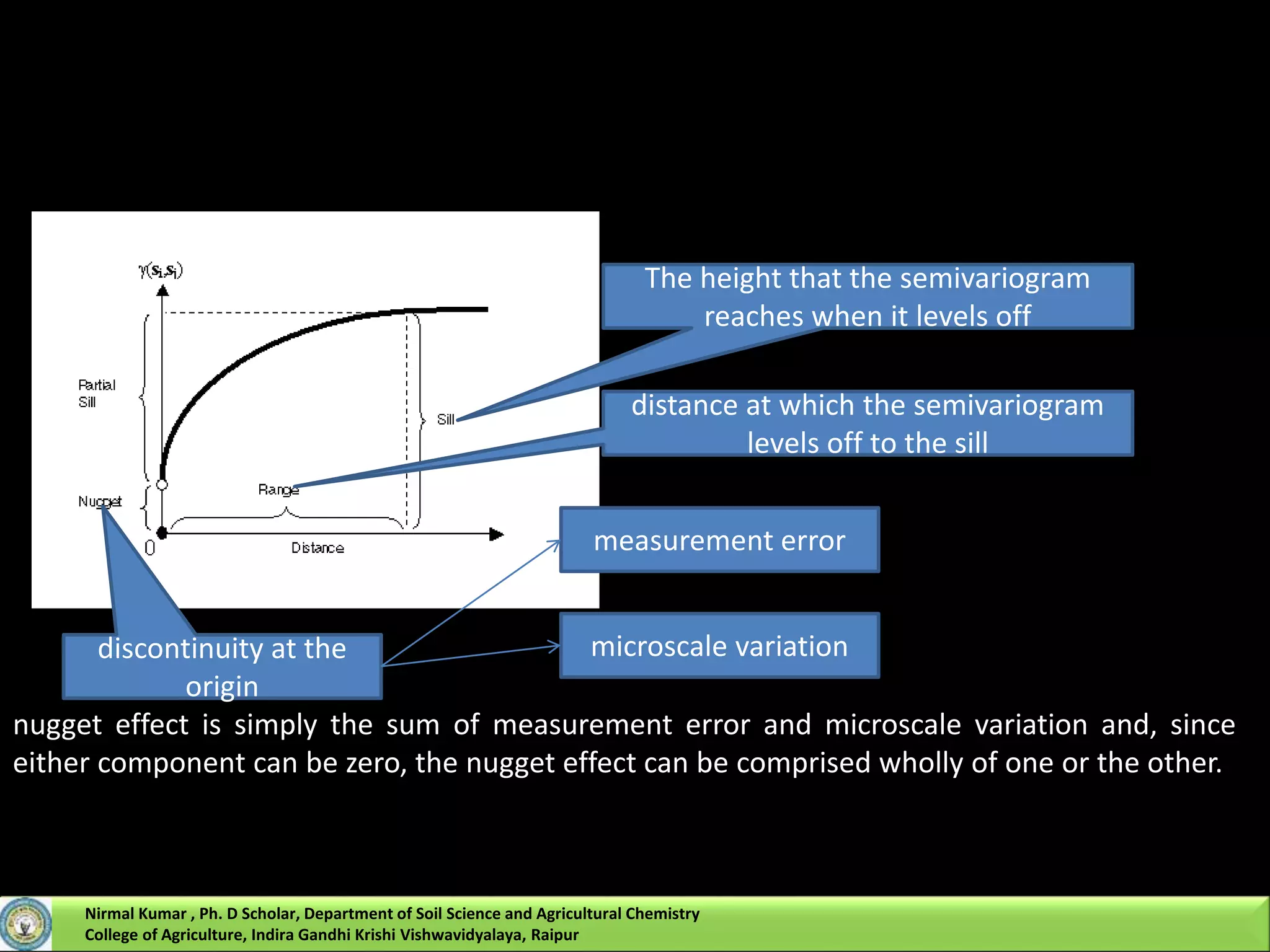
![Kriging
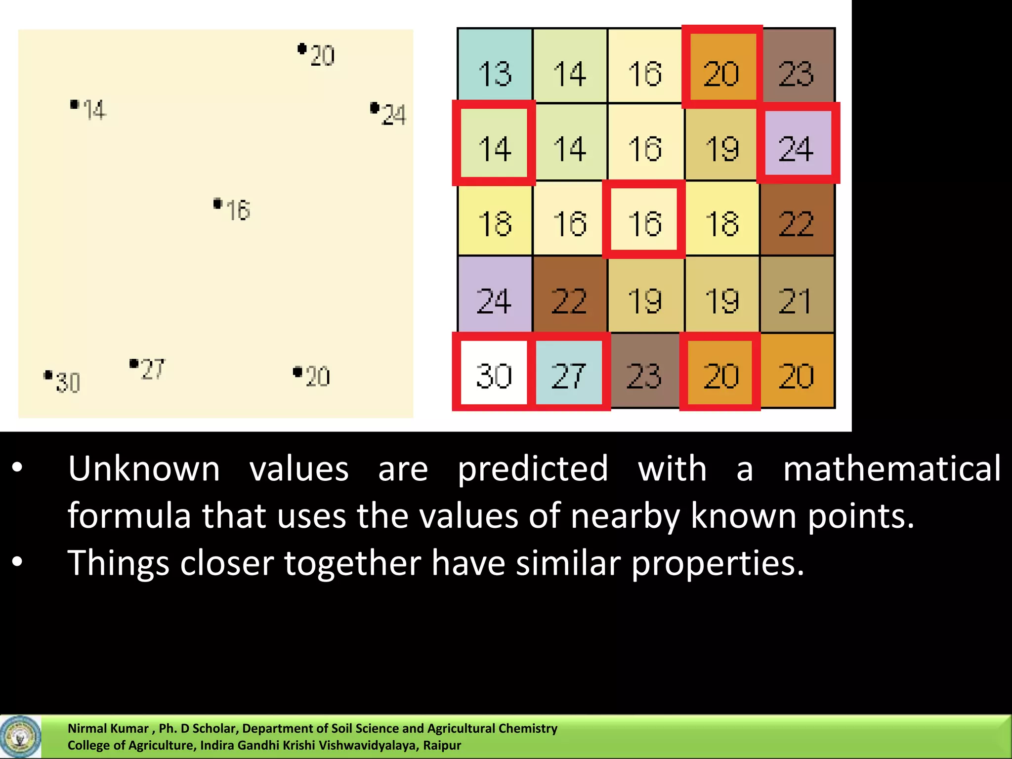
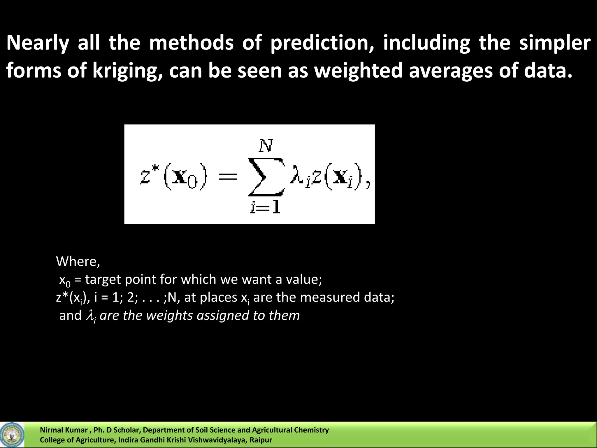
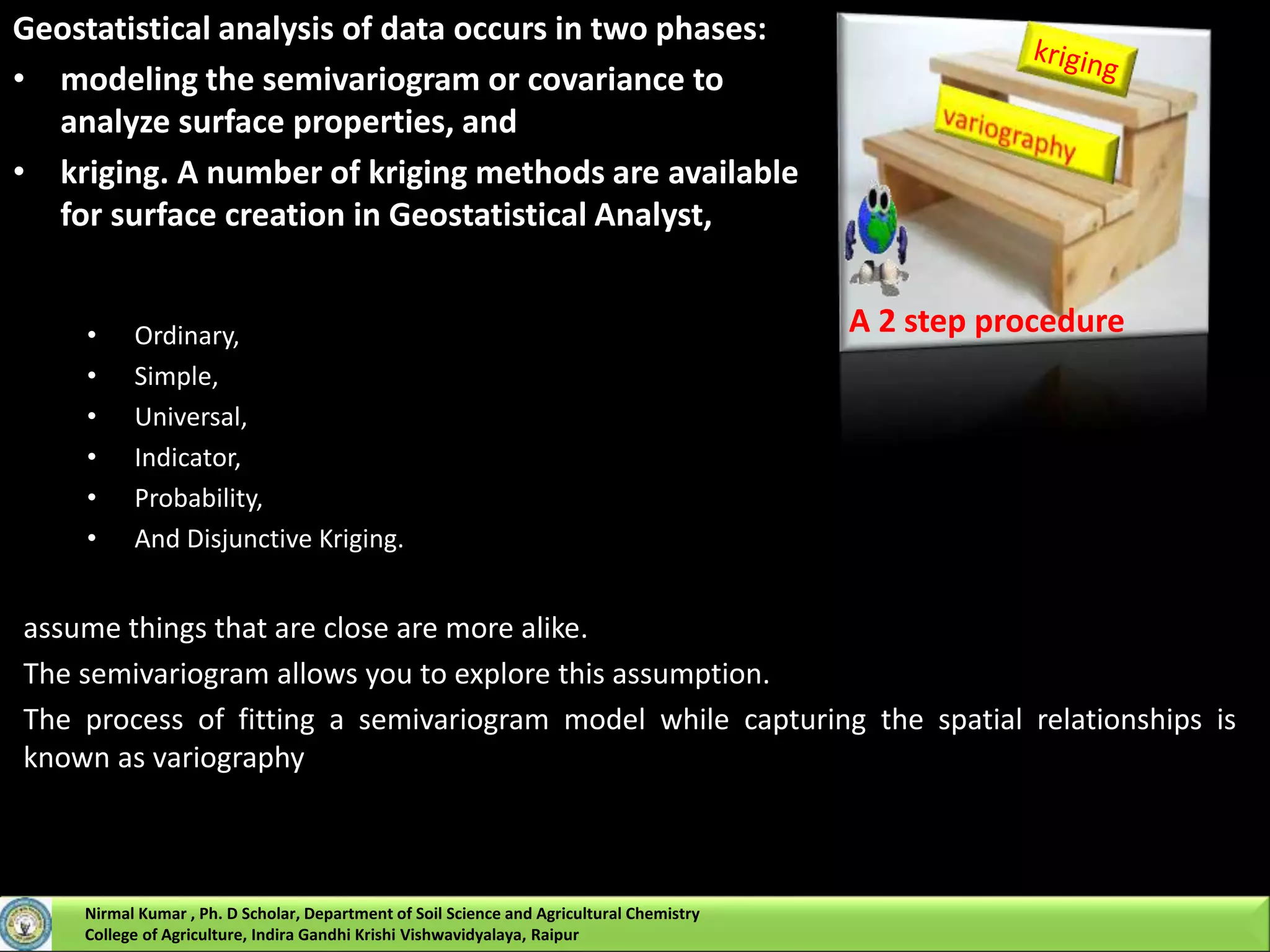
Like IDW interpolation, kriging forms weights from surrounding measured values to predict
values at unmeasured locations.
As with IDW interpolation, the closest measured values usually have the most influence.
However, IDW uses a simple algorithm based on distance, but kriging weights come from a
semivariogram that was developed by viewing the spatial structure of the data.
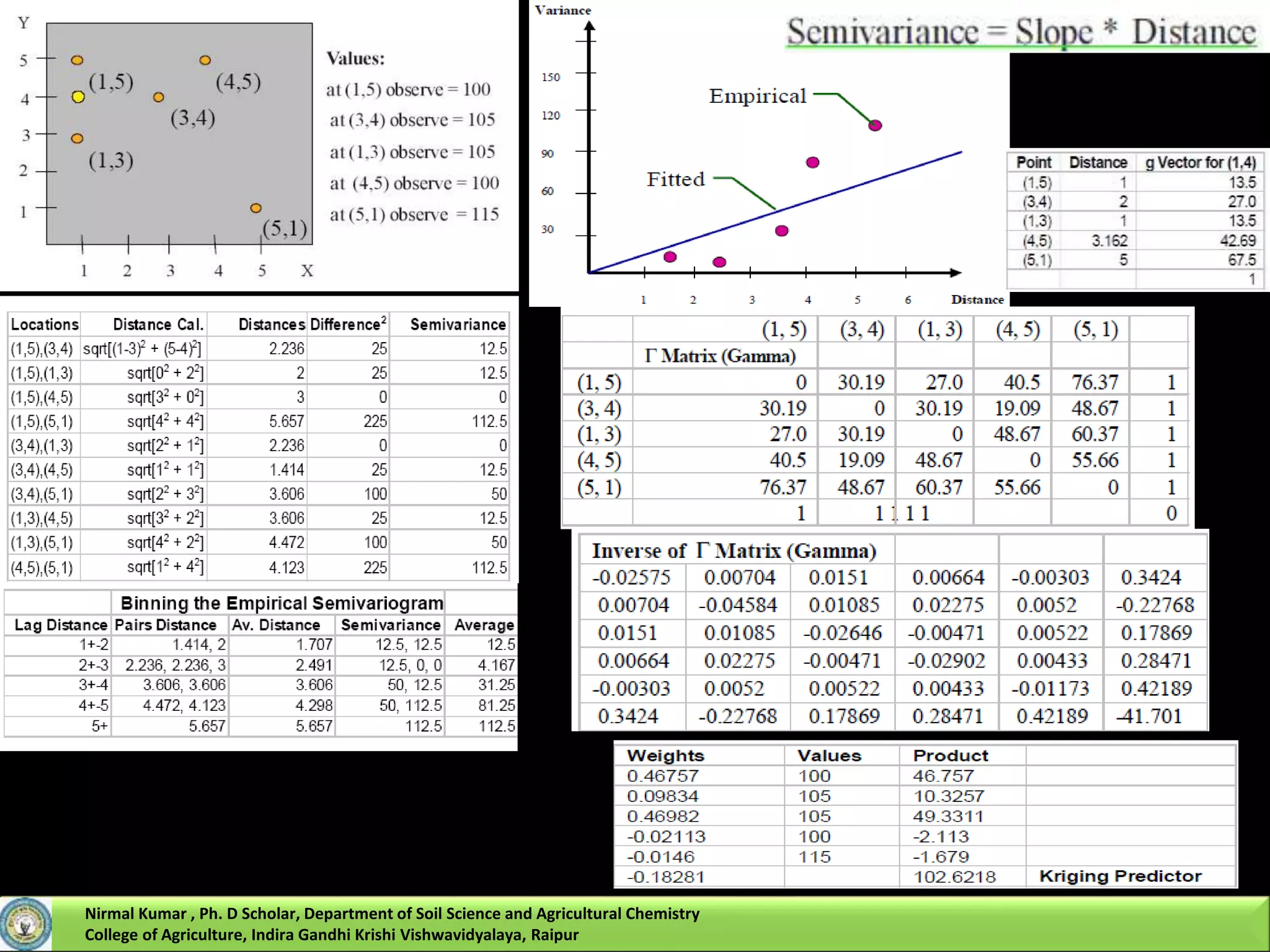
1. Create the Г – matrix and g-vector,
2. Calculate weights ʎ, and
3. Make a prediction
The key step in kriging is to estimate the n weighting factors for locations that neighbor the
unsampled location where interpolation is to occur.
a set of N+1 simultaneous equations with N+1 unknowns (the N weighting factors and the
undetermined Lagrangian multiplier).
Where,
[Г] is an N+1 by N+1 matrix of semivariogram values between measured locations,
[ʎ] is an N+1 by 1 matrix of weighting factors and the Lagrangian multiplier, and
[g] is an N+1 by 1 matrix of semivariogram values between the interpolated location and its neighboring
locations.
Nirmal Kumar , Ph. D Scholar, Department of Soil Science and Agricultural Chemistry
College of Agriculture, Indira Gandhi Krishi Vishwavidyalaya, Raipur](https://image.slidesharecdn.com/geostaticticsforsoilnutrientmapping-170529081040/75/Geostatictics-for-soil-nutrient-mapping-28-2048.jpg)


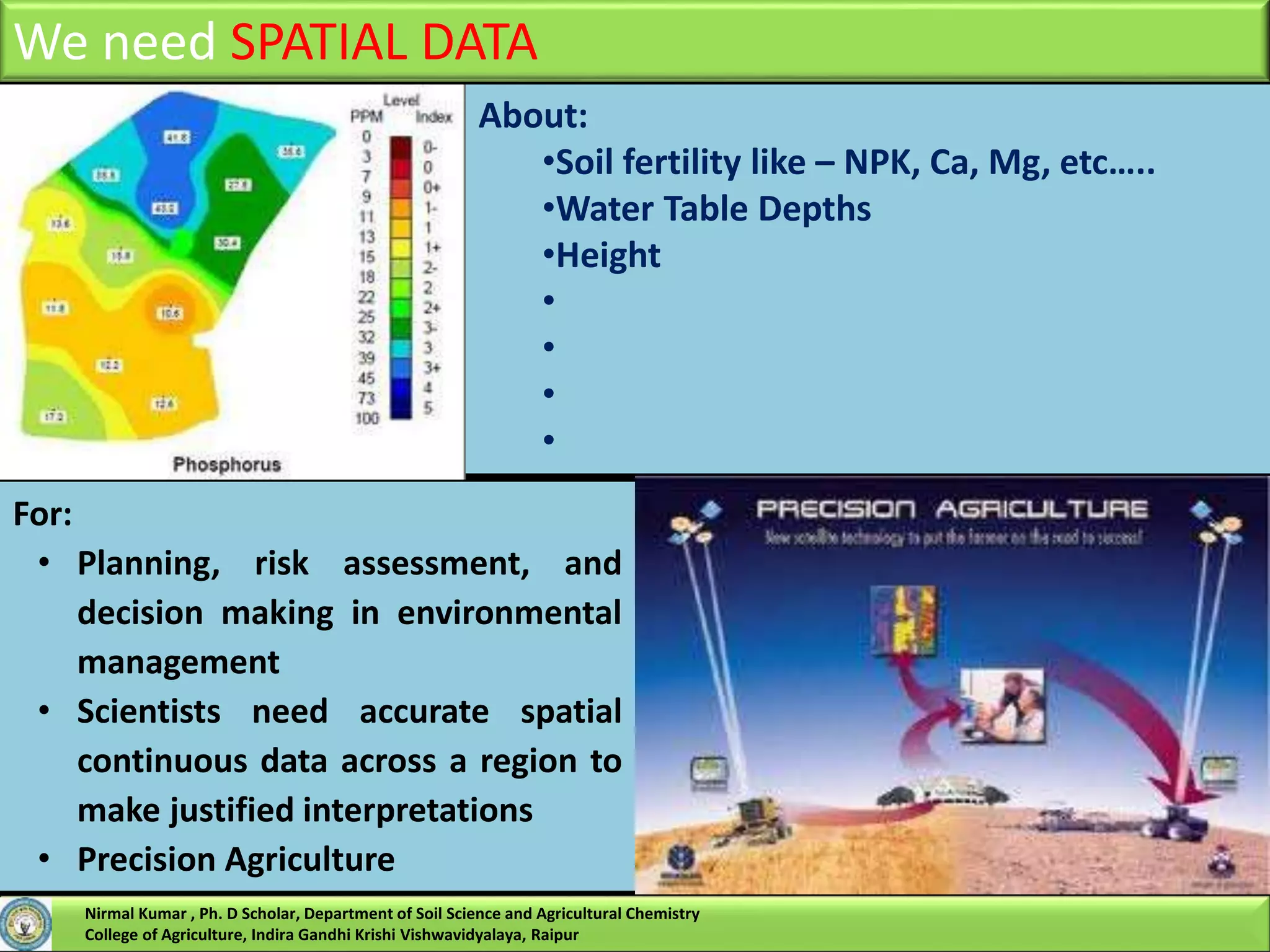
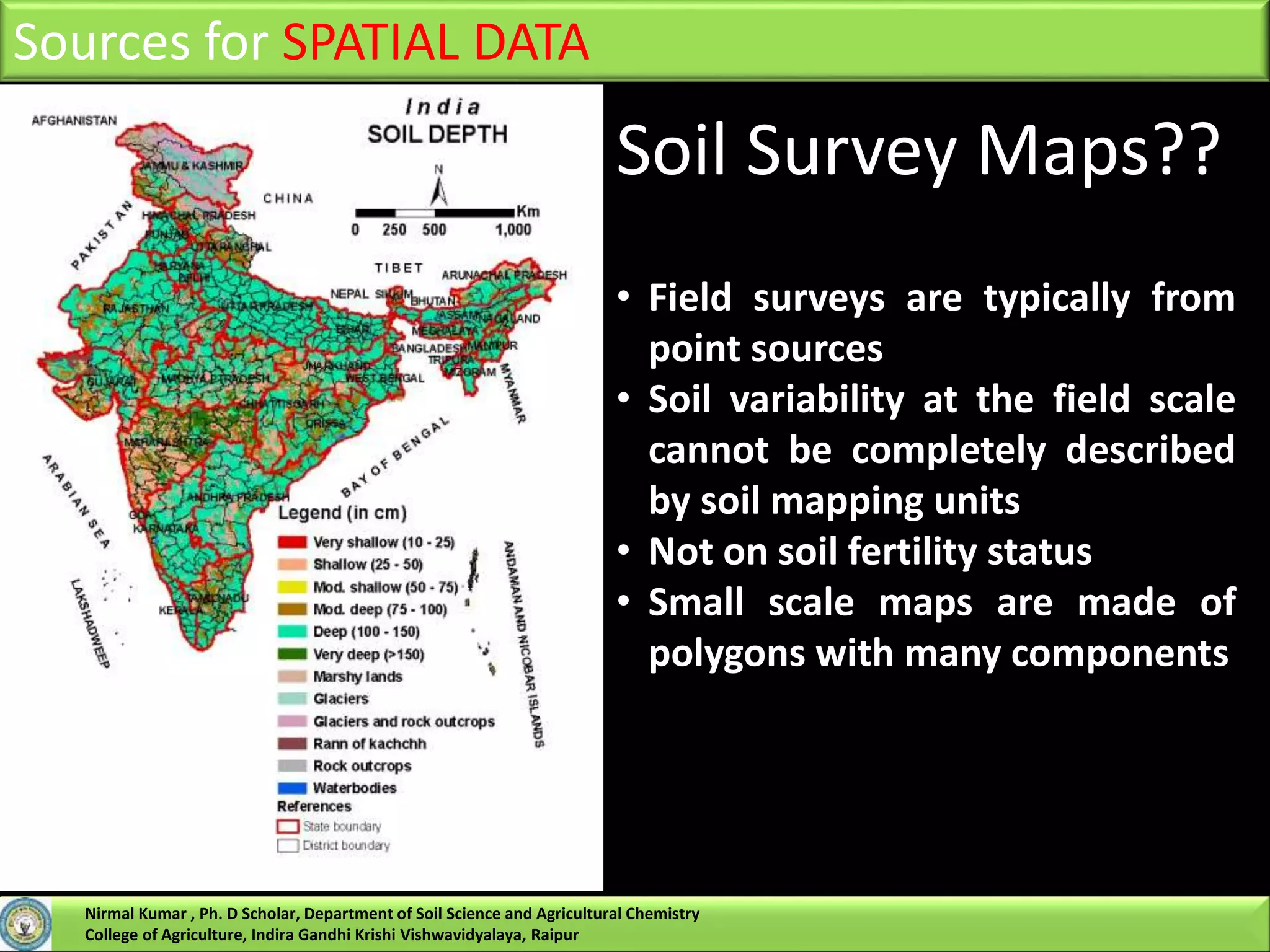
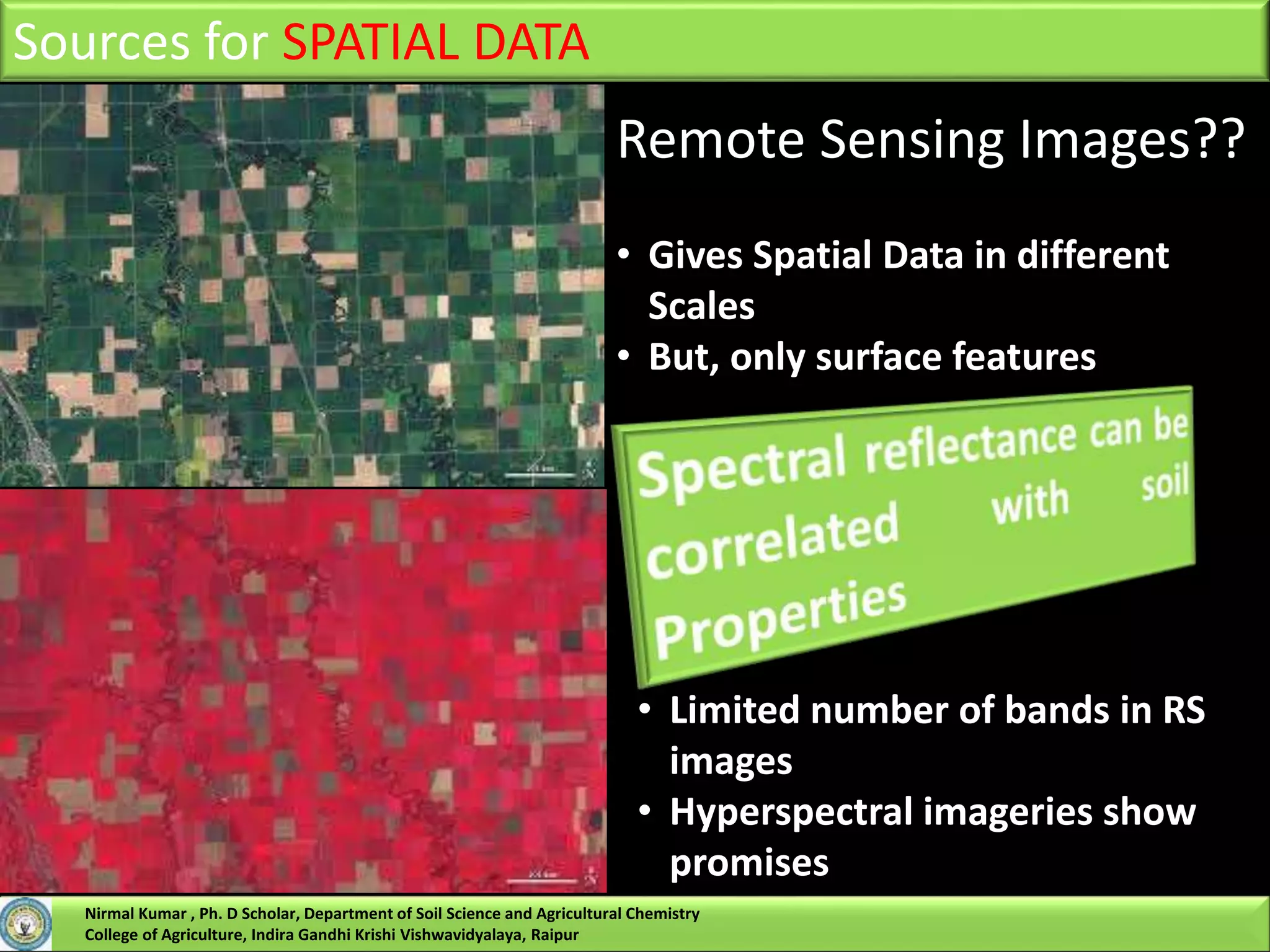
Nirmal Kumar, a PhD scholar, discusses spatial interpolation methods for soil nutrient mapping. Spatial data on soil properties is needed for planning, risk assessment, and precision agriculture but soil surveys only provide point data and remote sensing provides limited subsurface data. Various interpolation methods can be used to estimate values between data points, including inverse distance weighting and geostatistical kriging. Kriging uses a semivariogram to model spatial correlation and estimate weights for surrounding measurement points to predict values at unsampled locations. The presentation compares different spatial interpolation methods and issues to consider for accurate soil nutrient mapping.