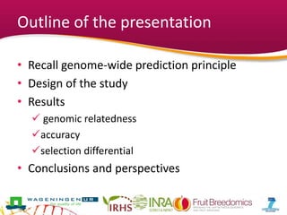
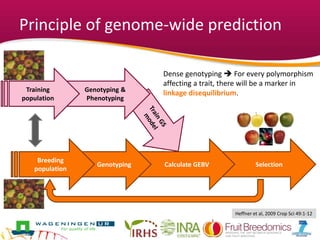
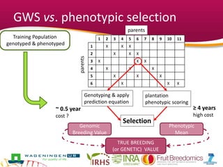
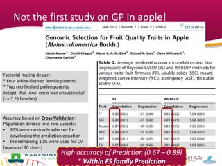
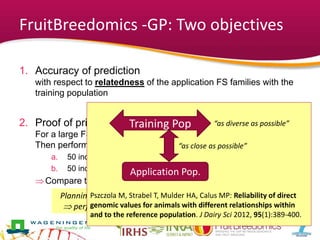
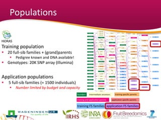
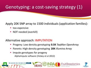
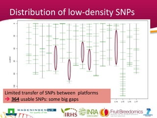
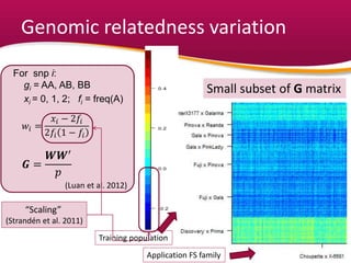
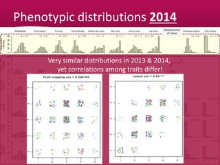
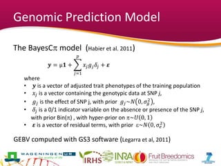
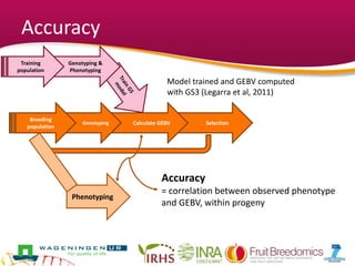
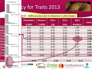
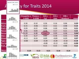
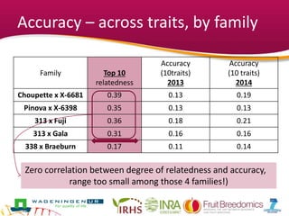
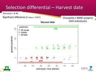
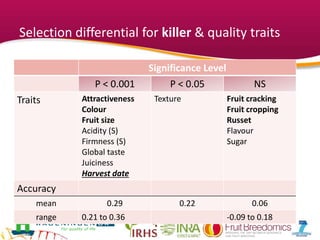
This document summarizes a two-year pilot study on genomic selection in apple breeding. The study involved genotyping and phenotyping a training population of 20 full-sib families and 5 application families. Genomic prediction models were developed and used to calculate genomic estimated breeding values (GEBV) for traits like fruit quality, size, and disease resistance. The accuracy of genomic prediction varied among traits from poor to moderate, and selection differentials based on GEBV were significant for several traits. The study provides a proof of concept for genomic selection in apple breeding but highlights the need for further research on prediction accuracy across multiple years and environments.

1. Genomic selection in apple:
A two years pilot study on
quantitative and ordinal traits
Hélène Muranty & Marco Bink

2. Acknowledgements
 Genotypic data
 Michela Troggio (FEM)
 Eric van de Weg (WUR)
 Mario Di Guardo (FEM-WUR)
 Elisa Banchi (FEM)
 Riccardo Velasco (FEM)
 Piergiorgio Stevanato (U. Padova)
 Design and analysis
 Hélène Muranty (INRA)
 Marco CAM Bink (WUR)
 Inès Ben Sadok (INRA)
 François Laurens (INRA)
 Phenotypic data
 Application (breeding) populations
 Mehdi Al Rifaï (INRA)
 François Lebreton (Novadi)
 Annemarie Auwerkerken (B3F)
 Erwin Collaerts (B3F)
 Training population
 Partners EU HiDRAS Project
 Phenotypic data integration
 Hans Jansen (WUR)
 Discussion
 Satish Kumar (PFR)

3. Outline of the presentation
• Recall genome-wide prediction principle
• Design of the study
• Results
 genomic relatedness
accuracy
selection differential
• Conclusions and perspectives

4. Principle of genome-wide prediction
SelectionCalculate GEBVGenotyping
Genotyping &
Phenotyping
Training
population
Breeding
population
Dense genotyping  For every polymorphism
affecting a trait, there will be a marker in
linkage disequilibrium.
Heffner et al, 2009 Crop Sci 49:1-12

5. GWS vs. phenotypic selection
1 2 3 4 5 6 7 8 9 10 11
1 X X X
2 X X X
3 X X X
4 X X X
5 X X X
6 X X X
parents
parents
plantation
phenotypic scoring
Selection
≥ 4 years
high cost
Genotyping & apply
prediction equation
~ 0.5 year
cost ?
Training Population
genotyped & phenotyped
Genomic
Breeding Value
Phenotypic
Mean
TRUE BREEDING
(or GENETIC) VALUE

6. Not the first study on GP in apple!
Factorial mating design:
* Four white-fleshed female parents
* Two red-fleshed pollen parents
except that one cross was unsuccessful
( 7 FS families)
Accuracy based on Cross Validation:
Population divided into two subsets:
• 90% were randomly selected for
developing the prediction equation
• the remaining 10% were used for CV
(repeated 10 times)
High accuracy of Prediction (0.67 – 0.89)
* Within FS family Prediction

7. FruitBreedomics -GP: Two objectives
1. Accuracy of prediction
with respect to relatedness of the application FS families with the
training population
2. Proof of principle
For a large FS family: Calculate Genomic Breeding Values(GBV).
Then perform phenotyping on:
a. 50 individuals with highest GBV
b. 50 individuals with lowest GBV
Compare the group (phenotypic) means
Planning too optimistic: GBVs not available in time!!
 perform phenotyping on many more individuals
Pszczola M, Strabel T, Mulder HA, Calus MP: Reliability of direct
genomic values for animals with different relationships within
and to the reference population. J Dairy Sci 2012, 95(1):389-400.
Training Pop
Application Pop.
“as diverse as possible”
“as close as possible”

8. Populations
founders training specific parents
training and application parents application specific parents
training FS families application FS families
intermediate ancestors
Delicious
GoldenDel
F2_26829-2-2
Jonathan
F_X-4598
AntonovkaOB
F_B8_34.16
DrOldenbu
Cox
Jefferies
PRI830-101
Wagenerap
RallsJan
RomBeauty
Clochard
O53T136
F_JamesGr
LadyWill
McIntosh
PRI14-126
PRI14-152
PRI14-510
F_Prima
X-4598
BVIII_34.16
Alkmene
Clivia
Winesap
X-4828
Idared
Fuji
Crandall
M_PRI668-100
KidsOrRed
Rubinette
Chantecler
F_Ill_#2
TN_R10A8
X-6823
JamesGr
F_Reka
Braeburn
PinkLady
F_Reanda
Telamon
PRI612-1
Prima
Z185
F_X-4355
Pinova
X-3188
PRI668-100
Gala
PRI672-3
ReiDuMans
Ill_#2
X-6417
Priam
Reka
Rewena
Pirol
Reanda
Discovery
TeBr
Florina
X-4355
X-3177
X-2771
RedWinter
X-6799
GranSmith
Coop-17
X-4638
X-3174
338
313
FuGa
GaCr
GaPi
RePir
FuPi
PiRea
DiPr
JoPr
X-6820
X-6681
X-3143
Galarina
X-6564
X-3263
RedWinterX3177
Baujade
X-3259
X-6679
X-6808
Dorianne
Choupette
B3F-fam2
B3F-fam1
B3F-fam4
X-6398
X-6683
X-3318
X-3305
12_O
I_BB
12_I
12_K
12_L
I_CC
Novadi-fam2
I_W
Novadi-fam1
I_M
12_F
12_J
I_J
12_P
12_N
HiDRAS
Training population
 20 full-sib families + (grand)parents
 Pedigree known and DNA available!
 Genotypes: 20K SNP array (Illumina)
Application populations
 5 full-sib families (= 1500 individuals)
 Number limited by budget and capacity

9. Genotyping: a cost-saving strategy (1)
Apply 20K SNP array to 1500 individuals (application families):
 too expensive
 NOT needed (overkill)
Alternative approach: IMPUTATION
 Progeny: Low density genotyping 0.5K TaqMan OpenArray
 Parents: High density genotyping 20K Illumina Array
 Impute genotypes for progeny
AlphaImpute software (Hickey et al 2012)

10. Distribution of low-density SNPs
Limited transfer of SNPs between platforms
 364 usable SNPs: some big gaps

11. Genomic relatedness variation
xi = 0, 1, 2; fi = freq(A)
𝑤𝑖 =
𝑥𝑖 − 2𝑓𝑖
2𝑓𝑖 1 − 𝑓𝑖
𝑮 =
𝑾𝑾′
𝑝
(Luan et al. 2012)
For snp i:
gi = AA, AB, BB Small subset of G matrix
Application FS family
Training population
“Scaling”
(Strandén et al. 2011)

12. Bigger subset of G matrix
Distribution
for a single individual of application family
to all individuals of the training population :

13. Relatedness
Choupette x
X-6681
Pinova x
X-6398
313 x
Fuji
313 x
Gala
338 x
Braeburn
Marker based
top 25% 0.14 0.17 0.18 0.16 0.08
top 5% 0.31 0.29 0.30 0.26 0.13
top 10 0.39 0.35 0.36 0.31 0.17
Pedigree based 0.11 0.19 0.16 0.22 0.03
Five application FS families to the training population
4 2 3 1 5
1 3 2 4 5
Different ranking and spacing!

14. Phenotypes
 Killer traits (scored at harvest)
 Fruit cropping, fruit size, pre-
harvest dropping
 Attractiveness, colour, russet,
cracking
 Fruit quality traits
 sensory assessment
firmness, crispness, juiciness,
flavour, sugar, acidity, texture,
global taste
 instrumental measurement
firmness, brix
Training population
 results from 3 years
 several sites (within Europe)
 771 to 963 individuals phenotyped
 adjusted means
Application populations
 results from 2013 harvest
 2 sites (1 per breeder)
 raw phenotypic values
HiDRAS

15. Phenotypic distributions 2013
Attractiveness
of colour

16. Phenotypic distributions 2014
Attractiveness
of colour
Very similar distributions in 2013 & 2014,
yet correlations among traits differ!

17. Genomic Prediction Model
The BayesC model (Habier et al. 2011)
𝒚 = µ𝟏 +
𝑗=1
𝑝
𝑥𝑗 𝑔𝑗 𝛿𝑗 + 𝜺
where
• 𝒚 is a vector of adjusted trait phenotypes of the training population
• 𝑥𝑗 is a vector containing the genotypic data at SNP j,
• 𝑔𝑗 is the effect of SNP j, with prior 𝑔𝑗~𝑁 0, 𝜎𝑔
2 ,
• 𝛿𝑗 is a 0/1 indicator variable on the absence or presence of the SNP j,
with prior Bin() , with hyper-prior on ~𝑈 0, 1
• 𝜺 is a vector of residual terms, with prior ~𝑁 0, 𝜎𝑒
2
GEBV computed with GS3 software (Legarra et al, 2011)

18. Accuracy
SelectionCalculate GEBVGenotyping
Genotyping &
Phenotyping
Training
population
Breeding
population
Phenotyping
Accuracy
= correlation between observed phenotype
and GEBV, within progeny
Model trained and GEBV computed
with GS3 (Legarra et al, 2011)

19. Accuracy for Traits 2013
Choupette x
X-6681
Pinova x
X-6398
313 x
Fuji
313 x
Gala
338 x
Braeburn
mean
Family size 662 172 269 109 178
Attractiveness 0.21 0.18 0.35 0.19 0.14 0.21
Fruit cropping 0.08 0.09 0.02 0.19 0.03 0.08
Fruit size 0.26 0.19 0.08 0.33 0.25 0.23
Percent russet 0.18 0.21 0.38 0.30 -0.06 0.20
Percent over colour 0.31 0.22 0.50 0.46 0.36 0.37
Over colour 0.34 0.17 0.44 0.49 0.32 0.35
Ground colour -0.03 0.12 0.09 -0.05 0.17 0.06
Type colour -0.06 0.00 -0.25 -0.23 -0.14 -0.14
Pre-harvest dropping 0.02 -0.06 -0.02 -0.02
Fruit cracking -0.09 -0.05 0.13 -0.02 0.07 0.01
Mean_10Traits 0.13 0.13 0.18 0.16 0.11
LOW accuracy due to skewness in phenotypes

20. Accuracy for Traits 2014
Choupette x
X-6681
Pinova x
X-6398
313 x
Fuji
313 x
Gala
338 x
Braeburn mean
Attractiveness 0.30 0.10 0.36 0.16 0.06 0.20
Fruit cropping 0.15 -0.06 0.13 0.21 0.08 0.10
Fruit size 0.29 0.22 0.08 0.20 0.26 0.21
Percent russet 0.36 0.04 0.34 0.17 0.21 0.22
Percent over colour 0.29 0.30 0.67 0.59 0.36 0.44
Over colour 0.34 0.27 0.65 0.58 0.35 0.44
Ground colour -0.11 0.24 0.09 -0.09 0.20 0.07
Type colour -0.08 -0.09 -0.28 -0.28 -0.18 -0.18
Pre-harvest dropping -0.08 -0.13 -0.03 -0.08
Fruit_cracking 0.15 0.15 0.06 0.12
Mean_10Traits 0.19 0.13 0.21 0.16 0.14

21. Accuracy – across traits, by family
Family Top 10
relatedness
Accuracy
(10traits)
2013
Accuracy
(10 traits)
2014
Choupette x X-6681 0.39 0.13 0.19
Pinova x X-6398 0.35 0.13 0.13
313 x Fuji 0.36 0.18 0.21
313 x Gala 0.31 0.16 0.16
338 x Braeburn 0.17 0.11 0.14
Zero correlation between degree of relatedness and accuracy,
range too small among those 4 families!)

22. Selection differential – Harvest date
Accuracy = 0.36
Choupette x X6681 progeny
(543 individuals)
Significant difference (P-value < 0.001)
298
279

23. Selection differential for killer & quality traits
Significance Level
P < 0.001 P < 0.05 NS
Traits Attractiveness
Colour
Fruit size
Acidity (S)
Firmness (S)
Global taste
Juiciness
Harvest date
Texture Fruit cracking
Fruit cropping
Russet
Flavour
Sugar
Accuracy
mean 0.29 0.22 0.06
range 0.21 to 0.36 -0.09 to 0.18

24. Conclusions & perspectives
• A full-sized experiment pilot study
 application populations = progenies from breeders
 Cost-saving genotyping strategy + imputation
• Limited transfer between genotyping platforms – revisit & assess
imputation
• manuscript on GP for killer traits to be submitted
• Accuracy of Genomic Prediction
• Varies among traits (range from poor to moderate/good)
• Major impact from trait distributions (skewness, ordinal)
• Range in genomic relatedness limited: No correlation with accuracy
• Selection Response significant for several traits
• GP good at eliminating the worse & pontentially identifying the best
• Continue to study on accuracy of prediction
• multiple years (GxE)
• All traits (killer and quality traits)