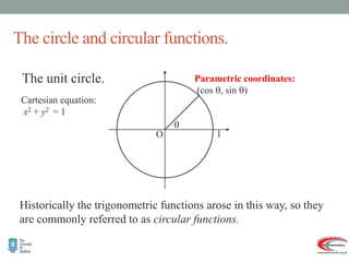
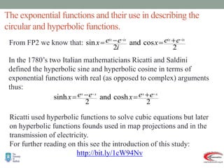
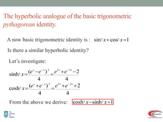
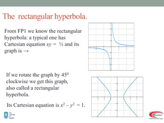
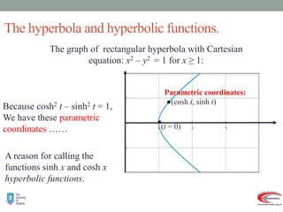
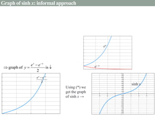
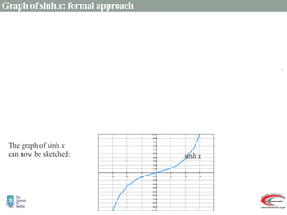
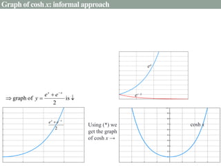
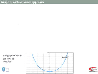
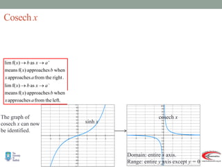
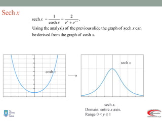
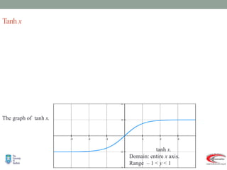
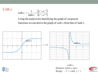
This document provides an overview of hyperbolic functions including: - Their definition in terms of exponential functions compared to circular/trigonometric functions defined using the unit circle. - Graphs and properties of the six main hyperbolic functions (sinh, cosh, tanh, sech, coth, cosech) derived using exponential definitions and relationships between functions. - Typical session structure includes introducing hyperbolic functions, defining the six functions, proving identities, and example exam questions.

1. FURTHERPURE3SKE
HYPERBOLICFUNCTIONS

2. Philosophy of the course
• The course does not aim to present a teaching plan for any of
the FP3 topics. This is left to your professional judgement as a
teacher.
• The course is more about presenting each topic in a way that
provides insights into the topic beyond the syllabus.
• In general the course will present the necessary knowledge and
skills to teach the Edexcel FP3 module effectively.
• Relevant examination problem solving techniques will be
demonstrated.

3. Session structure
• Section 1: Introduction to hyperbolic functions. How? Why?
When?
• Section 2: The six hyperbolic functions defined by the
exponential function; their graphs and properties.
• Section 3: Proofs of identities and solutions of equations
involving hyperbolic functions.
• Section 4: The inverses of the hyperbolic functions: graphs
properties and logarithmic equivalents.
• Section 5. Typical examination questions.

4. •Section 1: Introduction to
hyperbolic functions. How?
Why? When?

5. The circle and circular functions.
The unit circle.
O 1
Cartesian equation:
x2 + y2 = 1

Parametric coordinates:
(cos , sin )
Historically the trigonometric functions arose in this way, so they
are commonly referred to as circular functions.

6. The exponential functions and their use in describing the
circular and hyperbolic functions.
From FP2 we know that:
2
cos
and
2
sin
ix
ix
ix
ix e
e
x
i
e
e
x

 



In the 1780’s two Italian mathematicians Ricatti and Saldini
defined the hyperbolic sine and hyperbolic cosine in terms of
exponential functions with real (as opposed to complex) arguments
thus:
2
cosh
and
2
sinh
x
x
x
x e
e
x
e
e
x

 



Ricatti used hyperbolic functions to solve cubic equations but later
on hyperbolic functions founds used in map projections and in the
transmission of electricity.
For further reading on this see the introduction of this study:
http://bit.ly/1cW94Nv

7. From the above we derive:
The hyperbolic analogue of the basic trigonometric
pythagorean identity.
A now basic trigonometric identity is : 1
cos
sin 2
2 
 x
x
4
2
4
)
(
sinh
2
2
2
2






 x
x
x
x
e
e
e
e
x
Is there a similar hyperbolic identity?
Let’s investigate:
4
2
4
)
(
cosh
2
2
2
2






 x
x
x
x
e
e
e
e
x
1
sinh
cosh 2
2 
 x
x

8. The rectangular hyperbola.
Its Cartesian equation is x2 – y2 = 1.
If we rotate the graph by 450
clockwise we get this graph,
also called a rectangular
hyperbola.
From FP1 we know the rectangular
hyperbola: a typical one has
Cartesian equation xy = ½ and its
graph is →

9. The hyperbola and hyperbolic functions.
The graph of rectangular hyperbola with Cartesian
equation: x2 – y2 = 1 for x ≥ 1:
Parametric coordinates:
●(cosh t, sinh t)
Because cosh2 t – sinh2 t = 1,
We have these parametric
coordinates ……
●
(t = 0)
A reason for calling the
functions sinh x and cosh x
hyperbolic functions.

10. •Section 2: The six hyperbolic
functions defined by the
exponential function; their
graphs and properties.

11. Graph of sinh x: informal approach
.
0
for
sinh
of
graph
the
of
shape
the
find
to
need
just
we
So
(*)
origin
about the
symmetry
turn
2
1
has
sinh
of
graph
The
sinh
2
)
sinh(
.
2
sinh
that
noted
have
We











x
x
x
x
e
e
x
e
e
x
x
x
x
x
sinh x
:
are
0
for
and
of
graphs
The 

 
x
e
y
e
y x
x
ex
e– x





is
2
of
graph
x
x
e
e
y
2
x
x
e
e 

Using (*) we
get the graph
of sinh x →

12. Graph of sinh x: formal approach
points.
turning
no
has
sinh
so
,
0
2
)
(sinh
as
sinh
,
as
0
and
Since
0
for
graph
the
examine
only
need
we
So
origin.
about the
symmetry
turn
2
1
has
sinh
of
graph
The
sinh
2
)
sinh(
axis.
entire
the
is
sinh
of
domain
the
so
axis,
entire
the
is
of
or
of
domain
The
.
0
2
1
1
0
sinh
that
Note
.
2
sinh
seen that
have
We
x
e
e
x
dx
d
x
x
x
e
e
x
x
x
e
e
x
x
x
x
e
e
e
e
x
x
x
x
x
x
x
x
x
x
x





























sinh x
The graph of sinh x
can now be sketched:

13. Graph of cosh x: informal approach
.
0
for
cosh
of
graph
the
of
shape
the
find
to
need
just
we
So
(*)
0
about
symmetric
is
cosh
of
graph
The
cosh
2
)
cosh(
.
1
2
0
cosh
.
2
cosh
have
We
0
0















x
x
x
x
x
e
e
x
e
e
e
e
x
x
x
x
x
cosh x
:
are
0
for
and
of
graphs
The 

 
x
e
y
e
y x
x
ex
e– x





is
2
of
graph
x
x
e
e
y
2
x
x
e
e 

Using (*) we
get the graph
of cosh x →

14.  
1
cosh0
0
at
minimum
a
is
there
So
.
0
when
0
1
2
)
(cosh
0
1
when
0
2
)
(cosh
:
1.
is
cosh
of
range
1
1
2
2
2
2
2
Also
as
2
cosh
,
as
0
and
Since
.
0
for
cosh
examine
only
need
we
so
0,
about
symmetric
is
cosh
of
graph
The
cosh
2
)
cosh(
axis.
entire
the
is
cosh
of
domain
the
so
axis,
entire
the
is
of
or
of
domain
The
.
1
2
1
1
0
cosh
2
cosh
seen that
have
We
2
2
2
2
2
2































































y
x
x
e
e
x
dx
d
x
e
e
e
e
e
x
dx
d
ely
Alternativ
y
x
e
e
e
e
e
e
x
e
e
x
x
e
e
x
x
x
x
x
e
e
x
x
x
x
e
e
e
e
x
x
x
x
x
x
x
x
x
x
x
x
x
x
x
x
x
x
x
x
x
x
x
x
cosh x
The graph of cosh x
can now be
sketched:
Graph of cosh x: formal approach

15. Cosech x




















a
x
x
a
x
x
a
x
x
a
x
x
b
a
b
b
a
b
a
b
b
a
e
e
x
x x
x
as
0
)
f(
1
as
)
f(
as
)
f(
1
as
0
)
f(
)
1
,
(
at
Max.
0
),
,
(
at
Min.
)
1
,
(
at
Min.
0
),
,
(
at
Max.
:
following
the
note
merely
we
curves
reciprocal
graph
To
.
2
sinh
1
cosech
:
have
we
functions
.
with trig
As
)
f(
1
of
Graph
)
f(
of
Graph
x
x
sinh x
cosech x
.
left
the
from
approaches
when
approaches
)
f(
means
as
)
f(
lim
.
right
the
from
approaches
when
approaches
)
f(
means
as
)
f(
lim
a
x
b
x
a
x
b
x
a
x
b
x
a
x
b
x






The graph of
cosech x can now
be identified.
Domain: entire x axis.
Range: entire y axis except y = 0

16. Sech x
.
cosh
of
graph
the
from
derived
be
can
sech
of
graph
the
slide
previous
the
of
analysis
the
Using
.
2
cosh
1
sech
x
x
e
e
x
x x
x 



cosh x
sech x
sech x.
Domain: entire x axis.
Range 0 < y ≤ 1

17. Tanh x
 
 
 
 
 
 
 
 
 
 
 
 
     
   
.
1
0
tanh
Also
points.
turning
no
has
tanh
So
0
4
)
tanh
(
1
1
0
1
0
tanh
)
2
(
,
As
.
1
0
1
0
1
tanh
)
3
(
,
As
)
3
.....(
1
1
tanh
or
)
2
.....(
1
1
tanh
)
1
(
)
1
.........(
cosh
sinh
tanh
2
2
2
2
2
2
2
2




















































x
e
e
e
e
e
e
e
e
e
e
e
e
x
dx
d
x
x
x
x
e
e
x
e
e
x
e
e
e
e
x
x
x
x
x
x
x
x
x
x
x
x
x
x
x
x
x
x
x
x
x
x
x
e
e
e
e
x
x
x
x
tanh x.
Domain: entire x axis.
Range – 1 < y < 1
The graph of tanh x.

18. Coth x  
 
:
tanh
of
that
from
coth
of
graph
the
derive
can
we
functions
reciprocal
of
graph
the
g
identifyin
for
analysis
the
Using
tanh
1
coth
x
x
e
e
e
e
x
x x
x
x
x






coth x.
Domain: entire x axis.
Range: – 1 > y and y > 1
tanh x.
coth x.

19. Exercises: graphs of hyperbolic functions
?
3
13
2
sinh
3
equation
the
of
there
are
solutions
many
How
.
asymptotes
any
and
axes
the
of
intercepts
any
of
s
coordinate
the
giving
axes
of
set
same
on the
3
13
)
(
and
2
sinh
3
)
(
functions
the
of
graphs
Sketch the
2.
.
1
cosh
cosh
equation
the
of
solutions
of
number
the
State
axes.
of
set
same
on the
1
cosh
)
(
and
cosh
)
(
functions
the
of
graphs
Sketch the
1.
2
2
2
1
2
1
x
x
e
x
e
x
g
x
x
f
x
x
x
x
g
x
x
f











20. Exercises: graphs of hyperbolic functions – solutions.
.
1
cosh
cosh
equation
the
of
solutions
of
number
the
State
axes.
of
set
same
on the
1
cosh
)
(
and
cosh
)
(
functions
the
of
graphs
Sketch the
1.
2
1
2
1





x
x
x
x
g
x
x
f
Using transformations of the graph of y = cosh x we get:
x
x
f cosh
)
( 
1
cosh
)
( 2
1

 x
x
g
.
1
cosh
cosh
of
solutions
2
are
There
2
1

 x
x

21. Exercises: graphs of hyperbolic functions – solutions.
?
3
13
2
sinh
3
equation
the
of
there
are
solutions
many
How
.
asymptotes
any
and
axes
the
of
intercepts
any
of
s
coordinate
the
giving
axes
of
set
same
on the
3
13
)
(
and
2
sinh
3
)
(
functions
the
of
graphs
Sketch the
2.
2
2
x
x
e
x
e
x
g
x
x
f





Using transformations of the graph of y = ex and y =sinh x we get:
Asymptote y =13
x
x
f 2
sinh
3
)
( 
x
e
x
g 2
3
13
)
( 
 ●(0, 10)
)
0
,
ln
( 3
13
2
1

3
13
3
13
2
2
ln
2
3
13
0 




 x
e
e x
x
.
3
3
1
2
sinh
3
of
solution
1
is
There
2x
e
x 


22. •Section 3: Proofs of identities
and solutions of equations
involving hyperbolic functions.

23. Hyperbolic compound argument formulae: informal approach.
   
sinhes
two
of
product
sines
two
of
product 





































to
transfers
A
:
called
so
imply the
(2)
and
(1)
lines
that
Note
sinh
sinh
cosh
cosh
)
cosh(
Thus
)
2
...(
sinh
sinh
cosh
cosh
sinh
.
sinh
cosh
cosh
)
1
...(
sin
sin
cos
cos
)
cos(
also,
But,
)
cosh(
)
cos(
that
see
we
above
the
From
sinh
sinh
2
2
2
sin
cosh
2
2
2
cos
Then
and
Let
.
in
studied
is
that
something
and
acceptable
y
compeletel
is
This
angles.
complex
of
cosines
and
sines
consider
e
approach w
informal
In this
ones.
angle
compound
the
similar to
very
are
formulae
These
)
(
)
(
)
(
)
(
rule
Osborns
y
x
y
x
y
x
y
x
y
x
y
i
x
i
y
x
B
A
B
A
B
A
y
x
B
A
x
i
i
x
i
e
e
i
e
e
i
e
e
A
x
e
e
e
e
e
e
A
iy
B
ix
A
cs
mathemati
university
rical
trigonomet
x
x
ix
i
ix
i
iA
iA
x
x
ix
i
ix
i
iA
iA

24. Hyperbolic compound argument formulae: informal approach (contd).
same.
the
is
equivalent
hyperbolic
the
means
this
formula
angle
compound
trig
in the
sines
two
of
product
no
was
there
As
sinh
cosh
cosh
sinh
)
sinh(
Thus
)
sinh
cosh
cosh
(sinh
sinh
.
cosh
cosh
sinh
sin
cos
cos
sin
)
sin(
also,
But,
)
sinh(
)
sin(
sinh
sin
cosh
cos
:
facts
previous
the
use
We
and
for
formula
angle
compound
sine
he
consider t
Now
y
x
y
x
y
x
y
x
y
x
i
y
i
x
y
x
i
B
A
B
A
B
A
y
x
i
B
A
x
i
A
x
A
iy
B
ix
A



















25. Hyperbolic compound argument formulae: formal approach.
y
x
y
x
y
x
y
x
e
e
e
e
e
e
e
e
e
e
e
e
e
e
e
e
e
e
e
e
y
x
y
x
y
x
y
x
y
x
n
examinatio
y
x
y
x
y
x
y
x
y
x
y
x
y
x
y
x
y
x
y
x
y
x
y
x
y
y
x
x
y
y
x
x
sinh
sinh
cos
cosh
)
cosh(
Thus
)
cosh(
2
4
2
2
4
4
2
2
2
2
sinh
sinh
cos
cosh
:
work the
We
sinh
sinh
cos
cosh
)
cosh(
that
proof
the
is
Here
functions.
hyperbolic
of
s
definition
l
exponentia
the
using
by
but
angles
complex
of
cosines
and
sines
to
recourse
by
not
formulae
angle
compound
these
prove
to
has
one
papers
In
)
(

















































RHS
0
0
0
0
0
0
0
0
0

26. List of hyperbolic compound argument formulae.
)
1
sinh
cos
to
applied
rule
Osborns
(
1
sinh
cosh
:
outset)
at the
ed
(establish
7)
)
tanh
)
tanh(
note
and
5)
in
of
place
in
put
(
tanh
tanh
1
tanh
tanh
)
tanh(
)
6
tanh
tanh
1
tanh
tanh
)
tanh(
)
5
tanh
tanh
1
tanh
tanh
cosh
cosh
by
divide
now
:
sinh
sinh
cosh
cosh
sinh
cosh
cosh
sinh
)
cosh(
)
sinh(
)
tanh(
:
in
as
procedure
same
adopt the
we
equivalent
tanh
obtain the
To
get this)
we
3)
in
of
place
in
put
we
if
(
sinh
cosh
cosh
sinh
)
sinh(
)
4
sinh
cosh
cosh
sinh
)
sinh(
)
3
get this)
we
1)
in
of
place
in
put
we
if
(
sinh
sinh
cosh
cosh
)
cosh(
)
2
sinh
sinh
cosh
cosh
)
cosh(
)
1
2
2
2
2








































x
x
x
x
y
y
y
y
y
x
y
x
y
x
y
x
y
x
y
x
y
x
y
x
y
x
y
x
y
x
y
x
y
x
y
x
y
x
y
x
ry
trigonomet
y
y
y
x
y
x
y
x
y
x
y
x
y
x
y
y
y
x
y
x
y
x
y
x
y
x
y
x

27. Further hyperbolic identities: example 1.









 









 










 










 








x
e
e
e
e
e
e
e
e
x
x
x
x
x
x
x
x
x
x
x
x
2
cosh
2
1
2
2
1
4
2
2
1
2
2
1
cosh
2
:
Work the
:
Proof
.
1
cosh
2
2
cosh
that
prove
cosh
of
definition
l
exponentia
the
Using
2
2
2
2
2
2
2
2
2
RHS

28. Equations involving hyperbolic functions: example 2





























)
5
2
ln(
5
2
2
20
4
:
solution
one
have
we
,
0
As
2
20
4
0
1
)
(
4
)
(
4
1
4
2
2
2
sinh
:
Solution
.
of
e
exact valu
the
Find
.
2
sinh
2
2
x
e
e
e
e
e
e
e
e
e
e
e
x
x
x
x
x
x
x
x
x
x
x
x
x
x

29. Equations involving hyperbolic functions: example 3







































.
3
ln
3
1
ln
or
7
ln
3
1
or
7
0
)
1
3
)(
7
(
0
7
)
(
22
)
(
3
0
22
7
3
0
22
2
2
5
5
11
2
.
2
2
.
5
11
sinh
2
cosh
5
:
Solution
11
sinh
2
cosh
5
if
of
e
exact valu
the
Find
2
x
e
e
e
e
e
e
e
e
e
e
e
e
e
e
e
x
x
x
x
x
x
x
x
x
x
x
x
x
x
x
x
x
x
x
x

30. Equations involving hyperbolic functions: example 4
   







 







 















































2
5
3
ln
or
2
5
3
ln
2
5
3
0
1
3
3
2
3
cosh
1
cosh
as
ue
former val
reject
:
2
3
or
2
1
cosh
0
)
3
cosh
2
)(
1
cosh
2
(
0
3
cosh
4
cosh
4
0
cosh
cosh
4
)
1
cosh
(
3
0
cosh
cosh
4
sinh
3
0
1
cosh
4
cosh
sinh
.
3
0
1
sech
4
tanh
3
terms.
cosh
only
contains
it
that
so
equation
e
convert th
to
1
sinh
cosh
identity
the
use
Rather we
.
definition
l
exponentia
the
use
t
don'
we
so
term
squared
a
is
There
:
Solution
0
1
sech
4
tanh
3
if
of
e
exact valu
the
Find
2
2
2
2
2
2
2
2
2
2
2
2
x
e
e
e
e
e
x
x
x
x
x
x
x
x
x
x
x
x
x
x
x
x
x
x
x
x
x
x
x
x
x
x
x
x
x

31. Exercises: Identities and equations
1
2
1
that tanh
show
that
sinh
)
1
cosh(
Given
.
3
2
coth
2
cosech
if
of
e
exact valu
the
Find
.
2
.
sinh
sinh
cosh
cosh
)
cosh(
that
prove
ls,
exponentia
of
in terms
sinh
and
cosh
of
s
definition
the
from
Starting
1.
2
2











e
e
e
x
x
x
x
x
x
y
x
y
x
y
x
.

32. Exercises: Identities and equations – solutions.
.
sinh
sinh
cosh
cosh
)
cosh(
that
prove
ls,
exponentia
of
in terms
sinh
and
cosh
of
s
definition
the
from
Starting
1.
y
x
y
x
y
x 


.
y
x
y
x
y
x
y
x
e
e
e
e
e
e
e
e
e
e
e
e
e
e
e
e
e
e
e
e
y
x
y
x
y
x
y
x
y
x
y
x
y
x
y
x
y
x
y
x
y
x
y
x
y
x
y
x
y
y
x
x
y
y
x
x
sinh
sinh
cosh
cosh
)
cosh(
Thus
)
cosh(
2
4
2
2
4
4
2
2
2
2
sinh
sinh
cosh
cosh
)
(















































33. Exercises: Identities and equations – solutions,
2
coth
2
cosech
if
of
e
exact valu
the
Find
.
2 
 x
x
x
.
   
2
ln
2
1
ln
2
1
0
2
1
0
1
0
sinh
2
cosh
2
1
0
2
sinh
cosh
2
sinh
1
2
coth
2
cosech

































x
e
e
e
e
e
e
x
x
x
x
x
x
x
x
x
x
x
x
x

34. Exercises: Identities and equations – solutions.
   
   
   
   
  1
2
1
tanh
tanh
1
2
1
tanh
2
1
tanh
1
tanh
2
tanh
tanh
2
tanh
2
cosh
by
(1)
Dividing
)
1
........(
sinh
2
sinh
2
cosh
sinh
)
1
cosh(
So
2
sinh
2
cosh
1
sinh
sinh
1
cosh
cosh
)
1
cosh(
:
Solution
1
2
1
that tanh
show
that
sinh
)
1
cosh(
Given
.
3
2
2
2
2
2
2
1
1
1
1
1
1
1
1
1
1
1
1
1
1
1
1
2
2





















































e
e
e
x
x
e
e
e
x
e
e
x
e
x
e
e
x
e
e
x
e
e
x
e
e
x
x
e
e
x
e
e
x
x
x
e
e
x
e
e
x
x
x
x
e
e
e
x
x
x
.

35. •Section 4: The inverses of the
hyperbolic functions: graphs
properties and logarithmic
equivalents.

36. Arsinh x: the inverse of sinh x
sinh x
Evidently sinh x is a 1-1 function.
So no restriction of its domain is
required to determine its inverse.
We can find the graph of the
inverse, arsinh x, by reflecting the
graph of sinh x in y = x:
y = x
arsinh x
sinh x
The domain of arsinh x is the
entire x axis, its range the
entire y axis.

37. The logarithmic form of arsinh x
Arsinh x can be expressed in terms
of a logarithm. To see this we need
to do the following:
arsinh x
   
)
1
ln(
arsinh
:
s
other word
In
)
1
ln(
1
.
1
solution
reject the
we
0
As
.
0
1
so
,
1
Now
1
2
4
4
2
0
1
2
1
2
2
2
.
sinh
Then
.
arsinh
Let
2
2
2
2
2
2
2
2
2
2











































x
x
x
x
x
y
x
x
e
x
x
e
x
x
x
x
x
x
x
x
e
e
x
e
e
xe
e
e
x
e
e
x
y
x
x
y
y
y
y
y
y
y
y
y
y
y
y

38. Arcosh x: the inverse of cosh x
cosh x cosh x is not a 1-1
function.
So we need to
restrict its domain
to x ≥ 0 to consider
a 1-1 part →
We can find the graph of the
inverse, arcosh x, by reflecting the
graph of cosh x, x ≥ 0, in y = x:
y = x
arcosh x
cosh x, x ≥ 0
The domain of arcosh x is x ≥ 1,
its range y ≥ 0.
cosh x, x ≥ 0

39. The logarithmic form of arcosh x
arcosh x
   
   
 
  
 
 
 
 
       
 
1
ln
arcosh
Thus
.
0
fact that
the
o
contrary t
0
implies
option
This
1
1
1
,
0
1
ln
1
ln
1
ln
1
1
1
1
1
1
1
1
1
hold.
cannot
option
second
why the
see
to
algebra
some
do
to
need
we
Now
1
ln
or
1
ln
1
2
4
4
2
0
1
2
1
2
2
2
.
cosh
Then
.
0
,
1
,
arcosh
Let
2
2
2
1
2
2
2
2
2
2
2
2
2
2
2
2
2
2
2
2









































































x
x
x
y
y
y
x
x
x
x
x
x
x
x
x
x
x
x
x
x
x
x
x
x
x
x
x
x
x
x
x
y
x
x
y
x
x
x
x
e
e
x
e
e
xe
e
e
x
e
e
x
y
x
y
x
x
y
y
y
y
y
y
y
y
y
y
0
Arcosh x can be expressed in
terms of a logarithm. The
procedure is similar to one used
for arsinh x:

40. Artanh x: the inverse of tanh x
tanh x tanhh x is a 1-1 function.
So we do not need to
restrict its domain to
determine its inverse.
We find the graph of the inverse,
artanh x as before: by reflecting
the graph of tanh x in y = x:
y = x
artanh x
tanh x
The domain of artanh x is
– 1< x <1, its range the entire y axis.

41. The logarithmic form of artanh x
artanh x
 
   
1
1
,
1
1
ln
2
1
artanh
Thus
1
1
ln
2
1
1
1
ln
2
1
1
1
)
1
(
1
.
tanh
Then
.
1
1
,
artanh
Let
2
2
2
2
2
1
2
1






























































x
x
x
x
y
x
x
y
x
x
y
x
x
e
x
e
x
e
x
xe
e
e
e
e
x
e
e
e
e
x
y
x
x
x
y
y
y
y
y
y
y
y
y
y
y
y
y
Artanh x also has a logarithmic
form. The procedure to determine
it is as follows:

42. Exercises: Inverse hyperbolic functions







 




2
2
1
1
ln
arcosech
that
show
to
Q1
Use
2.
1
arsinh
as
written
be
can
arcosech
expression
that the
Show
cosech
of
inverse
the
is
arcosech
Given that
1.
x
x
x
x
y
x
y
x
x
x
.

43. Exercises: Inverse hyperbolic functions – solutions.
.
 







 



















































2
2
2
2
1
1
ln
arcosech
.
.
1
1
1
ln
1
arsinh
arcosech
(*)
So
1
ln
arsinh
that
know
We
......(*)
1
arsinh
arcosech
Q1
2.
1
arsinh
sinh
1
cosech
arcosech
1.
x
x
x
x
e
i
x
x
x
x
x
x
x
x
x
y
x
y
x
y
x
y
x
v
v
v
v
v
v

44. •Section 5. Typical examination
questions.

45. Example 1
 
 













2
4
2
4
2
4
2
2
2
1
2
1
2
1
2
2
cosh
Then
.
ln
k
k
e
e
e
e
e
e
x
k
e
k
x
x
x
x
x
x
x
x
.
2
1
2
cosh
then
,
0
,
ln
if
that
Show 2
4
k
k
x
k
k
x





46. Example 2
   
3
ln
2
1
3
ln
2
)
0
(
3
0
)
3
)(
1
9
(
0
3
26
9
0
3
26
9
6
26
3
3
6
26
3
3
3
13
2
3
3
13
2
sinh
3
2
2
2
2
2
2
2
2
4
4
2
4
2
2
2
2
2
2
2



































x
x
e
e
e
e
e
e
e
e
e
e
e
e
e
e
e
e
e
e
x
x
x
x
x
x
x
x
x
x
x
x
x
x
x
x
x
x
x
integer.
an
is
where
,
ln
2
1
form
in the
answer
your
giving
3
13
2
sinh
3
equation
the
Solve 2
k
k
e
x x


Exercises:graphsofhyperbolicfunctions.q2continuation

47. Example 3





































.
5
ln
5
1
ln
or
3
ln
5
1
or
3
0
)
1
5
)(
3
(
0
3
)
(
16
)
(
5
0
16
3
5
0
16
4
4
8
2
2
.
4
8
sinh
cosh
4
2
x
e
e
e
e
e
e
e
e
e
e
e
e
e
e
e
x
x
x
x
x
x
x
x
x
x
x
x
x
x
x
x
x
8
sinh
cosh
4
if
of
e
exact valu
the
Find 
 x
x
x

48. Example 4
.
logarithms
natural
as
answer
your
giving
cosh
5
3
cosh
solve
Hence
ii)
.
3
cosh
cosh
3
cosh
4
that
prove
to
ls
exponentia
of
in terms
cosh
of
definition
the
Use
i)
3
x
x
x
x
x
x



.
 
   
 
)
(continued
3
cosh
2
2
1
2
3
2
2
3
4
2
4
2
3
2
4
2
)
3
cosh
4
(
cosh
cosh
3
cosh
4
i)
3
3
3
3
2
2
2
2
2
2
2
2
3



















 











 

















 








 

















 







 
















x
e
e
e
e
e
e
e
e
e
e
e
e
e
e
e
e
e
e
e
e
e
e
e
e
x
x
x
x
x
x
x
x
x
x
x
x
x
x
x
x
x
x
x
x
x
x
x
x
x
x
x
x

49. Example 4
.
logarithms
natural
as
answer
your
giving
cosh
5
3
cosh
solve
Hence
ii)
.
3
cosh
cosh
3
cosh
4
that
prove
to
ls
exponentia
of
in terms
cosh
of
definition
the
Use
i)
3
x
x
x
x
x
x



.
   
)
1
2
ln(
or
)
1
2
ln(
1
2
2
4
8
2
2
0
1
2
2
2
2
)
1
(cosh
2
cosh
0
)
2
(cosh
cosh
4
0
cosh
8
cosh
4
cosh
5
cosh
3
cosh
4
cosh
5
3
cosh
ii)
2
2
3
3































x
e
e
e
e
e
x
x
x
x
x
x
x
x
x
x
x
x
x
x
x
x

50. Example 5
.
1
1
ln
arsech
,
1
0
for
that,
show
ls
exponentia
of
in terms
sech
of
definition
the
Using
ii)
1
1
ln
1
1
ln
that
hence,
and,
1
1
1
1
that
show
1
0
If
i)
2
2
2
2
2







 











 










 








x
x
x
x
x
x
x
x
x
x
x
x
x
x
.
 
  
 
 
 
 
 
  )
(continued
1
1
2
4
4
2
0
2
2
2
2
1
0
where
,
sech
Then
.
0
arsech
Let
ii)
1
1
ln
1
1
ln
1
1
1
1
1
1
1
1
1
1
1
1
1
1
1
1
1
1
1
1
i)
2
2
2
2
2
2
1
2
2
2
2
2
2
2
2
2
2
2
x
x
x
x
e
x
e
e
x
e
x
xe
e
e
x
e
e
x
x
x
y
y
x
x
x
x
x
x
x
x
x
x
x
x
x
x
x
x
x
x
x
x
x
x
x
y
y
y
y
y
y
y
y
y
































 










 









 




























.
1
0
when
1
1
1
that
assume
question
this
In
2




 x
x
x

51. Example 5
.
 







 










 




















 










 

















x
x
x
x
x
y
x
x
e
x
x
e
y
x
x
x
x
x
x
y
x
x
e
x
x
x
x
e
x
e
e
x
y
y
y
y
y
y
2
2
2
2
2
2
2
2
2
2
2
1
1
ln
arsech
1
1
ln
or
1
1
Thus
.
1
1
reject
,
0
As
1
1
1
as
0,
1
1
ln
1
1
ln
1
1
1
1
2
4
4
2
0
2
.....
.
1
1
ln
arsech
,
1
0
for
that,
show
ls
exponentia
of
in terms
sech
or
cosh
of
definition
the
Using
ii)
1
1
ln
1
1
ln
that
hence,
and,
1
1
1
1
that
show
1
0
If
i)
2
2
2
2
2







 











 










 








x
x
x
x
x
x
x
x
x
x
x
x
x
x
x
.
1
0
when
1
1
1
that
assume
question
this
In
2




 x
x
x