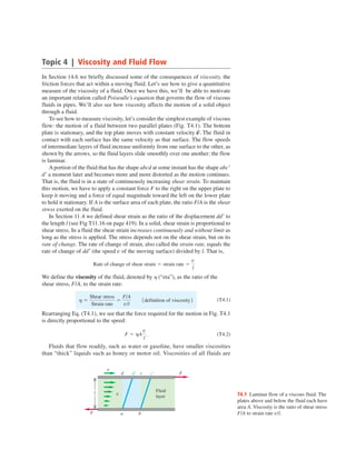
Topic 4 | Viscosity and Fluid Flow
In Section 14.6 we briefly discussed some of the consequences of viscosity, the
friction forces that act within a moving fluid. Let’s see how to give a quantitative
measure of the viscosity of a fluid. Once we have this, we’ll be able to motivate
an important relation called Poiseulle’s equation that governs the flow of viscous
fluids in pipes. We’ll also see how viscosity affects the motion of a solid object
through a fluid.
    To see how to measure viscosity, let’s consider the simplest example of viscous
flow: the motion of a fluid between two parallel plates (Fig. T4.1). The bottom
plate is stationary, and the top plate moves with constant velocity µ. The fluid in
contact with each surface has the same velocity as that surface. The flow speeds
of intermediate layers of fluid increase uniformly from one surface to the other, as
shown by the arrows, so the fluid layers slide smoothly over one another; the flow
is laminar.
    A portion of the fluid that has the shape abcd at some instant has the shape abcr
dr a moment later and becomes more and more distorted as the motion continues.
That is, the fluid is in a state of continuously increasing shear strain. To maintain
this motion, we have to apply a constant force F to the right on the upper plate to
keep it moving and a force of equal magnitude toward the left on the lower plate
to hold it stationary. If A is the surface area of each plate, the ratio F/A is the shear
stress exerted on the fluid.
    In Section 11.4 we defined shear strain as the ratio of the displacement ddr to
the length l (see Fig T11.16 on page 419). In a solid, shear strain is proportional to
shear stress. In a fluid the shear strain increases continuously and without limit as
long as the stress is applied. The stress depends not on the shear strain, but on its
rate of change. The rate of change of strain, also called the strain rate, equals the
rate of change of dd′ (the speed v of the moving surface) divided by l. That is,
                                                                               v
                          Rate of change of shear strain 5 strain rate 5
                                                                               l
We define the viscosity of the fluid, denoted by h (“eta”), as the ratio of the
shear stress, F/A, to the strain rate:

                      Shear stress   F/A
                 h5                5                 1 definition of viscosity 2   (T4.1)
                       Strain rate   v/l
Rearranging Eq. (T4.1), we see that the force required for the motion in Fig. T4.1
is directly proportional to the speed:
                                                   v
                                             F 5 hA .                              (T4.2)
                                                   l
   Fluids that flow readily, such as water or gasoline, have smaller viscosities
than “thick” liquids such as honey or motor oil. Viscosities of all fluids are

                                v
                                         d     d9 c      c9             F


                                                              Fluid
                          l          v                                                      T4.1 Laminar flow of a viscous fluid. The
                                                              layer
                                                                                            plates above and below the fluid each have
                                                                                            area A. Viscosity is the ratio of shear stress
                      F                  a       b                                          F/A to strain rate v/l.
strongly temperature dependent, increasing for gases and decreasing for liquids as
                                               the temperature increases. An important goal in the design of oils for engine lubri-
                                               cation is to reduce the temperature variation of viscosity as much as possible.
                                                  From Eq. (T4.1) the unit of viscosity is that of force times distance, divided by
                                               area times speed. The SI unit is
                                                                       1 N # m/ 3 m2 # 1 m/s 2 4 5 1 N # s/m2 5 1 Pa # s.

                                               The corresponding cgs unit, 1 dyn # s/cm2, is the only viscosity unit in common
                                               use; it is called a poise, in honor of the French scientist Jean Louis Marie
                                               Poiseuille (pronounced “pwa-zoo-yuh”):
                                                                         1 poise 5 1 dyn # s/cm2 5 1021 N # s/m2.
                                               The centipoise and the micropoise are also used. The viscosity of water is 1.79
                                               centipoise at 0°C and 0.28 centipoise at 100°C. Viscosities of lubricating oils are
                                               typically 1 to 10 poise, and the viscosity of air at 20°C is 181 micropoise.
                                                  For a Newtonian fluid the viscosity h is independent of the speed v, and from
                                               Eq. (T4.2) the force F is directly proportional to the speed. Fluids that are sus-
    R                                          pensions or dispersions are often non-Newtonian in their viscous behavior. One
                                v vs. r        example is blood, which is a suspension of corpuscles in a liquid. As the strain rate
                                               increases, the corpuscles deform and become preferentially oriented to facilitate
                                               flow, causing h to decrease. The fluids that lubricate human joints show similar
                                               behavior.
T4.2 Velocity profile for a viscous fluid in      Figure T4.2 shows the flow speed profile for laminar flow of a viscous fluid in
a cylindrical pipe.                            a long cylindrical pipe. The speed is greatest along the axis and zero at the pipe
                                               walls. The motion is like a lot of concentric tubes sliding relative to one another,
                                               with the central tube moving fastest and the outermost tube at rest. By applying
                                               Eq. (T4.1) to a cylindrical fluid element, we could derive an equation describing
                                               the speed profile. We’ll omit the details; the flow speed v at a distance r from the
                                               axis of a pipe with radius R is
                                                                                   p1 2 p2
                                                                              v5             1 R2 2 r2 2 ,                    (T4.3)
                                                                                     4hL
                                               where p1 and p2 are the pressures at the two ends of a pipe with length L. The
                                               speed at any point is proportional to the change of pressure per unit length, 1 p2 2
                                               p2 2 p1 2 /L or dp/dx, called the pressure gradient. (The flow is always in the
                                               direction of decreasing pressure.) To find the total volume flow rate through the
                                               pipe, we consider a ring with inner radius r, outer radius r 1 dr, and cross-section
                                               area dA 5 2pr dr. The volume flow rate through this element is vdA; the total
                                               volume flow rate is found by integrating from r 5 0 to r 5 R The result is

                                                                 dV
                                                                 dt
                                                                    5
                                                                      8 h1 21
                                                                      p R 4 p1 2 p2
                                                                               L        2     1 Poiseuille’s equation 2       (T4.4)


                                                  This relation was first derived by Poiseuille and is called Poiseuille’s equa-
                                               tion. The volume flow rate is inversely proportional to viscosity, as we would
                                               expect. It is also proportional to the pressure gradient 1 p2 2 p1 2 /L, and it varies
                                               as the fourth power of the radius R. If we double R, the flow rate increases by a
                                               factor of 16. This relation is important for the design of plumbing systems and
                                               hypodermic needles. Needle size is much more important than thumb pressure in
                                               determining the flow rate from the needle; doubling the needle diameter has the
                                               same effect as increasing the thumb force sixteenfold. Similarly, blood flow in
                                               arteries and veins can be controlled over a wide range by relatively small changes
in diameter, an important temperature-control mechanism in warm-blooded ani-
mals. Relatively slight narrowing of arteries due to arteriosclerosis can result in
elevated blood pressure and added strain on the heart muscle.
    One more useful relation in viscous fluid flow is the expression for the force F
exerted on a sphere of radius r moving with speed v through a fluid with viscos-
ity h. When the flow is laminar, the relationship is simple:
                                 F 5 6phrv        1 Stokes’s law 2                      (T4.5)
We encountered this kind of velocity-proportional force in Section 5.3. Equation
(T4.5) is called Stokes’s law.


     Example
       T4.1              Terminal speed in a viscous fluid
Derive an expression for the terminal speed vt of a sphere falling in
a viscous fluid in terms of the sphere’s radius r and density and
the fluid viscosity h, assuming that the flow is laminar so that
Stokes’s law is valid.

 SOLUTION                                                                                                         Fbuoyancy
                                                                                                      Fvisc
As in Example 5.20 in Section 5.3, the terminal speed is reached                                              r       r

when the total force is zero, including the weight of the sphere, the                                  vt
viscous retarding force, and the buoyant force (Fig. T4.3). Let r
and rr be the densities of the sphere and of the fluid, respectively.                                             w

                                    3 pr rg,
                                    4   3
The weight of the sphere is then               and the buoyant force is                                r9, h
3 pr rrg. At
4   3
               terminal speed,
          vSFy 5 Fbouyancy 1 Fvisc 1 1 2mg 2                              T4.3 A sphere falling in a viscous fluid reaches a terminal speed
                    4                   4                                 when the sum of the forces acting on it is zero.
                  5 pr 3rrg 1 6phrvt 2 pr 3rg 5 0,
                    3                   3
                    2 r 2g
               vt 5        1 r 2 rr 2 .                                   terminal speeds in air. He used these drops to measure the charge of
                    9 h                                                   an individual electron.
    We can use this formula to measure the viscosity of a fluid. Or,          The terminal speed for a water droplet of radius 1025 m in air is
if we know the viscosity, we can determine the radius of the sphere       of the order of 1 cm/s; the Stokes’s-law force is what keeps clouds
(or the approximate sizes of other small particles) by measuring the      in the air. At higher speeds the flow often becomes turbulent, and
terminal speed. Robert Millikan used this method to determine the         Stokes’s law is no longer valid. In air the drag force at highway
radii of very small electrically charged oil drops by observing their     speeds is approximately proportional to v2. We discussed the appli-
                                                                          cations of this relation to skydiving in Section 5.3 and to air drag of
                                                                          a moving automobile in Topic 2 (Automotive Power).

Viscosity and fluid flow

  • 1.
    Topic 4 |Viscosity and Fluid Flow In Section 14.6 we briefly discussed some of the consequences of viscosity, the friction forces that act within a moving fluid. Let’s see how to give a quantitative measure of the viscosity of a fluid. Once we have this, we’ll be able to motivate an important relation called Poiseulle’s equation that governs the flow of viscous fluids in pipes. We’ll also see how viscosity affects the motion of a solid object through a fluid. To see how to measure viscosity, let’s consider the simplest example of viscous flow: the motion of a fluid between two parallel plates (Fig. T4.1). The bottom plate is stationary, and the top plate moves with constant velocity µ. The fluid in contact with each surface has the same velocity as that surface. The flow speeds of intermediate layers of fluid increase uniformly from one surface to the other, as shown by the arrows, so the fluid layers slide smoothly over one another; the flow is laminar. A portion of the fluid that has the shape abcd at some instant has the shape abcr dr a moment later and becomes more and more distorted as the motion continues. That is, the fluid is in a state of continuously increasing shear strain. To maintain this motion, we have to apply a constant force F to the right on the upper plate to keep it moving and a force of equal magnitude toward the left on the lower plate to hold it stationary. If A is the surface area of each plate, the ratio F/A is the shear stress exerted on the fluid. In Section 11.4 we defined shear strain as the ratio of the displacement ddr to the length l (see Fig T11.16 on page 419). In a solid, shear strain is proportional to shear stress. In a fluid the shear strain increases continuously and without limit as long as the stress is applied. The stress depends not on the shear strain, but on its rate of change. The rate of change of strain, also called the strain rate, equals the rate of change of dd′ (the speed v of the moving surface) divided by l. That is, v Rate of change of shear strain 5 strain rate 5 l We define the viscosity of the fluid, denoted by h (“eta”), as the ratio of the shear stress, F/A, to the strain rate: Shear stress F/A h5 5 1 definition of viscosity 2 (T4.1) Strain rate v/l Rearranging Eq. (T4.1), we see that the force required for the motion in Fig. T4.1 is directly proportional to the speed: v F 5 hA . (T4.2) l Fluids that flow readily, such as water or gasoline, have smaller viscosities than “thick” liquids such as honey or motor oil. Viscosities of all fluids are v d d9 c c9 F Fluid l v T4.1 Laminar flow of a viscous fluid. The layer plates above and below the fluid each have area A. Viscosity is the ratio of shear stress F a b F/A to strain rate v/l.
  • 2.
    strongly temperature dependent,increasing for gases and decreasing for liquids as the temperature increases. An important goal in the design of oils for engine lubri- cation is to reduce the temperature variation of viscosity as much as possible. From Eq. (T4.1) the unit of viscosity is that of force times distance, divided by area times speed. The SI unit is 1 N # m/ 3 m2 # 1 m/s 2 4 5 1 N # s/m2 5 1 Pa # s. The corresponding cgs unit, 1 dyn # s/cm2, is the only viscosity unit in common use; it is called a poise, in honor of the French scientist Jean Louis Marie Poiseuille (pronounced “pwa-zoo-yuh”): 1 poise 5 1 dyn # s/cm2 5 1021 N # s/m2. The centipoise and the micropoise are also used. The viscosity of water is 1.79 centipoise at 0°C and 0.28 centipoise at 100°C. Viscosities of lubricating oils are typically 1 to 10 poise, and the viscosity of air at 20°C is 181 micropoise. For a Newtonian fluid the viscosity h is independent of the speed v, and from Eq. (T4.2) the force F is directly proportional to the speed. Fluids that are sus- R pensions or dispersions are often non-Newtonian in their viscous behavior. One v vs. r example is blood, which is a suspension of corpuscles in a liquid. As the strain rate increases, the corpuscles deform and become preferentially oriented to facilitate flow, causing h to decrease. The fluids that lubricate human joints show similar behavior. T4.2 Velocity profile for a viscous fluid in Figure T4.2 shows the flow speed profile for laminar flow of a viscous fluid in a cylindrical pipe. a long cylindrical pipe. The speed is greatest along the axis and zero at the pipe walls. The motion is like a lot of concentric tubes sliding relative to one another, with the central tube moving fastest and the outermost tube at rest. By applying Eq. (T4.1) to a cylindrical fluid element, we could derive an equation describing the speed profile. We’ll omit the details; the flow speed v at a distance r from the axis of a pipe with radius R is p1 2 p2 v5 1 R2 2 r2 2 , (T4.3) 4hL where p1 and p2 are the pressures at the two ends of a pipe with length L. The speed at any point is proportional to the change of pressure per unit length, 1 p2 2 p2 2 p1 2 /L or dp/dx, called the pressure gradient. (The flow is always in the direction of decreasing pressure.) To find the total volume flow rate through the pipe, we consider a ring with inner radius r, outer radius r 1 dr, and cross-section area dA 5 2pr dr. The volume flow rate through this element is vdA; the total volume flow rate is found by integrating from r 5 0 to r 5 R The result is dV dt 5 8 h1 21 p R 4 p1 2 p2 L 2 1 Poiseuille’s equation 2 (T4.4) This relation was first derived by Poiseuille and is called Poiseuille’s equa- tion. The volume flow rate is inversely proportional to viscosity, as we would expect. It is also proportional to the pressure gradient 1 p2 2 p1 2 /L, and it varies as the fourth power of the radius R. If we double R, the flow rate increases by a factor of 16. This relation is important for the design of plumbing systems and hypodermic needles. Needle size is much more important than thumb pressure in determining the flow rate from the needle; doubling the needle diameter has the same effect as increasing the thumb force sixteenfold. Similarly, blood flow in arteries and veins can be controlled over a wide range by relatively small changes
  • 3.
    in diameter, animportant temperature-control mechanism in warm-blooded ani- mals. Relatively slight narrowing of arteries due to arteriosclerosis can result in elevated blood pressure and added strain on the heart muscle. One more useful relation in viscous fluid flow is the expression for the force F exerted on a sphere of radius r moving with speed v through a fluid with viscos- ity h. When the flow is laminar, the relationship is simple: F 5 6phrv 1 Stokes’s law 2 (T4.5) We encountered this kind of velocity-proportional force in Section 5.3. Equation (T4.5) is called Stokes’s law. Example T4.1 Terminal speed in a viscous fluid Derive an expression for the terminal speed vt of a sphere falling in a viscous fluid in terms of the sphere’s radius r and density and the fluid viscosity h, assuming that the flow is laminar so that Stokes’s law is valid. SOLUTION Fbuoyancy Fvisc As in Example 5.20 in Section 5.3, the terminal speed is reached r r when the total force is zero, including the weight of the sphere, the vt viscous retarding force, and the buoyant force (Fig. T4.3). Let r and rr be the densities of the sphere and of the fluid, respectively. w 3 pr rg, 4 3 The weight of the sphere is then and the buoyant force is r9, h 3 pr rrg. At 4 3 terminal speed, vSFy 5 Fbouyancy 1 Fvisc 1 1 2mg 2 T4.3 A sphere falling in a viscous fluid reaches a terminal speed 4 4 when the sum of the forces acting on it is zero. 5 pr 3rrg 1 6phrvt 2 pr 3rg 5 0, 3 3 2 r 2g vt 5 1 r 2 rr 2 . terminal speeds in air. He used these drops to measure the charge of 9 h an individual electron. We can use this formula to measure the viscosity of a fluid. Or, The terminal speed for a water droplet of radius 1025 m in air is if we know the viscosity, we can determine the radius of the sphere of the order of 1 cm/s; the Stokes’s-law force is what keeps clouds (or the approximate sizes of other small particles) by measuring the in the air. At higher speeds the flow often becomes turbulent, and terminal speed. Robert Millikan used this method to determine the Stokes’s law is no longer valid. In air the drag force at highway radii of very small electrically charged oil drops by observing their speeds is approximately proportional to v2. We discussed the appli- cations of this relation to skydiving in Section 5.3 and to air drag of a moving automobile in Topic 2 (Automotive Power).