Downloaded 112 times
![FLUID KINEMATICS
Kinematics deal with motion of fluid without any reference to cause of motion i.e., force.
The fluid flow is analysed by using two techniques.
1. Langrangian technique
2. Eulerian technique
In Langrangian technique, single fluid particle is taken and the behaviour of this particle is analysed at different
instances of time.
In Eulerian technique, certain section is taken and fluid flow is analysed at that section.
Different types of fluid flow
Steady & Unsteady flow
A flow is said to be steady flow when fluid properties do not change at any cross section at any given time,
otherwise flow is unsteady.
𝐹𝑜𝑟 𝑆𝑡𝑒𝑎𝑑𝑦 𝑓𝑙𝑜𝑤 → [
𝑑𝑣
𝑑𝑡
]
𝑔𝑖𝑣𝑒𝑛 𝑠𝑒𝑐𝑡𝑖𝑜𝑛
= 0 & [
𝑑𝜌
𝑑𝑡
]
𝑔𝑖𝑣𝑒𝑛 𝑠𝑒𝑐𝑡𝑖𝑜𝑛
= 0
Uniform & non-uniform flow
A flow is said to be uniform when fluid properties especially velocity don’t change with space at any given instant
of time, otherwise the flow is non-uniform.
𝐹𝑜𝑟 𝑈𝑛𝑖𝑓𝑜𝑟𝑚 𝑓𝑙𝑜𝑤 → [
𝑑𝑣
𝑑𝑠(𝑥, 𝑦, 𝑧)
]
𝑔𝑖𝑣𝑒𝑛 𝑡𝑖𝑚𝑒
= 0 {𝑠 = 𝑠𝑝𝑎𝑐𝑒(𝑥, 𝑦, 𝑧)}
Laminar & Turbulent flow
In laminar flow fluid particles move in the form of layers, with one layer sliding over the other layer. Laminar flow
generally occurs at low velocities.
In turbulent flow, fluid particles move in highly disorganized manner, leading to rapid mixing of particles.
Turbulent flow generally occurs at high velocities.
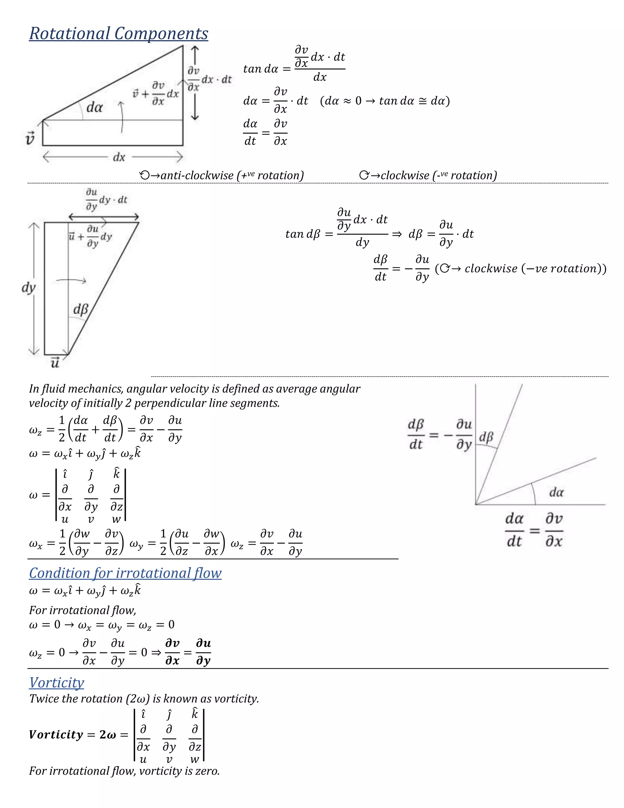
Rotational & Irrotational flow
A flow is said to be rotational flow when fluid particles rotate about their own mass centres, otherwise the flow is
irrotational.
Rotation is possible when there is a tangential force, these tangential forces are associated with viscous fluids.
Therefore, real fluids are generally rotational fluids and ideal fluids are irrotational fluids.
Internal & External flows
When the fluid flows through confined passage (Ex- flow of fluid through pipes, ducts) then it is internal flow.
When the fluid flow through unconfined passage (Ex- Flow of fluid (air) over aircraft wing) then flow is external
flow.
Categorization of flow
1. One-dimensional flow
2. Two-dimensional flow
3. Three-dimensional flow
Flow can never be 1-D, because of viscosity.
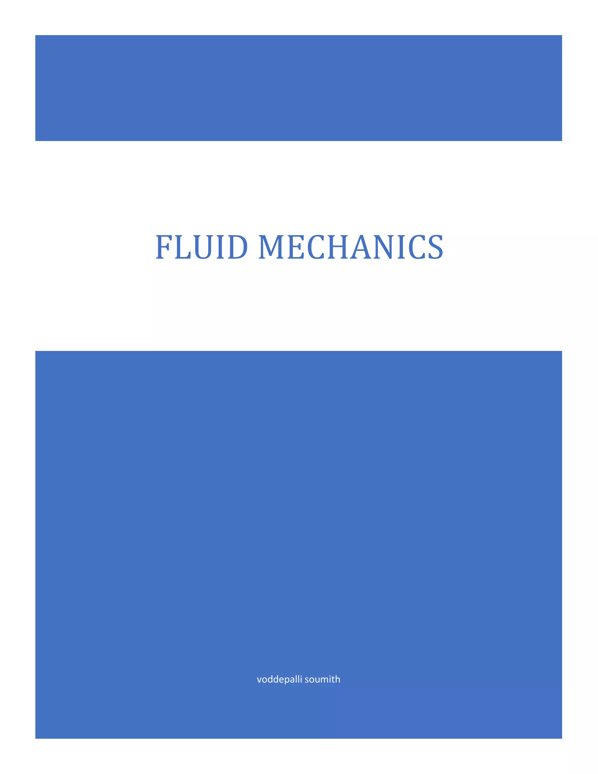
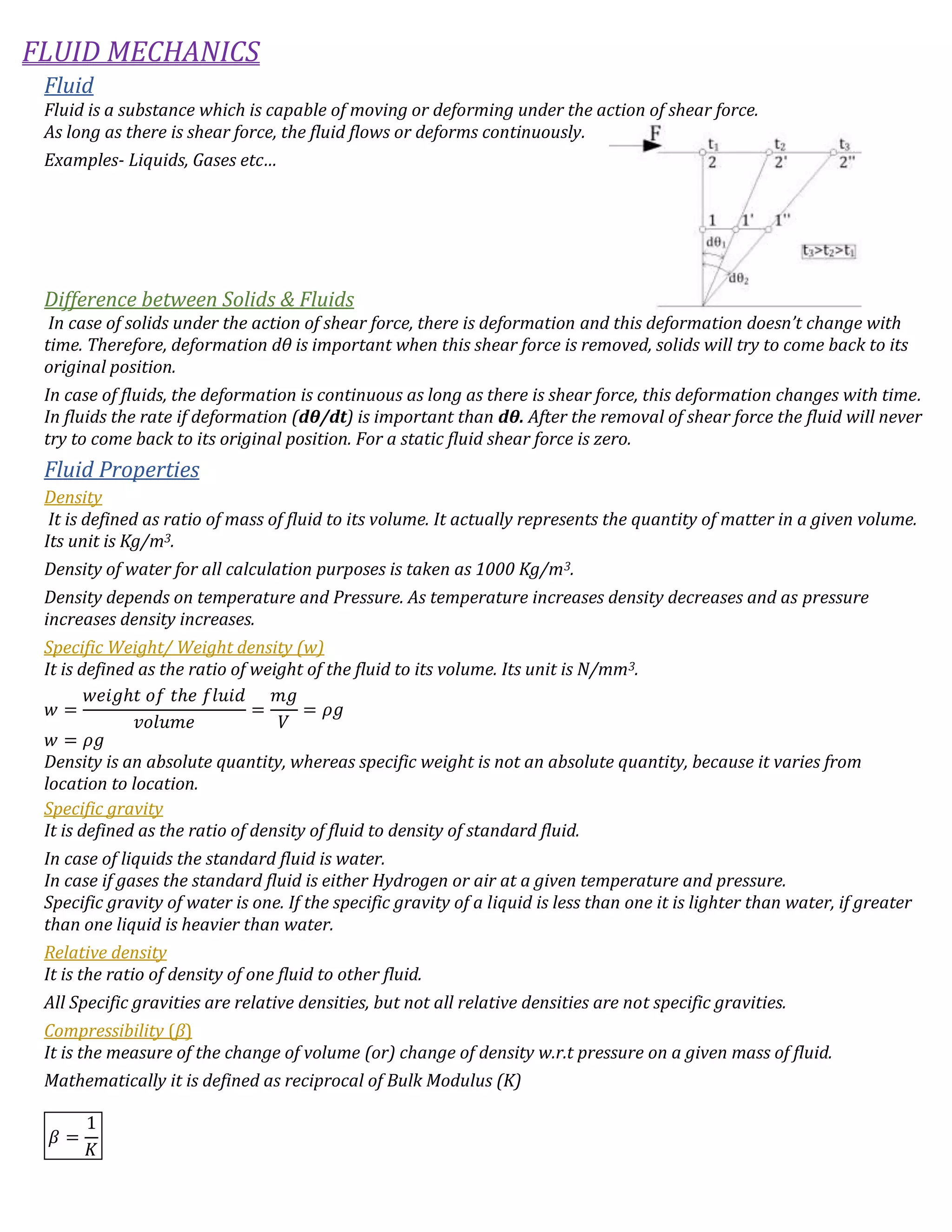
Stream line
It is an imaginary line or curve drawn in space such that a tangent drawn to it at any point gives velocity vector.
Stream line gives direction of flow as there is no component of velocity in perpendicular direction there is no flow
across the stream line, there is flow only along the stream line. Stream line gives instantaneous snapshot of a flow
pattern. It has no time history. No two stream lines can intersect because velocity is unique at any given instant of
time at a particular time.](https://image.slidesharecdn.com/fluidmechanicsfinal-180307190704/75/Fluid-mechanics-notes-for-gate-3-2048.jpg)

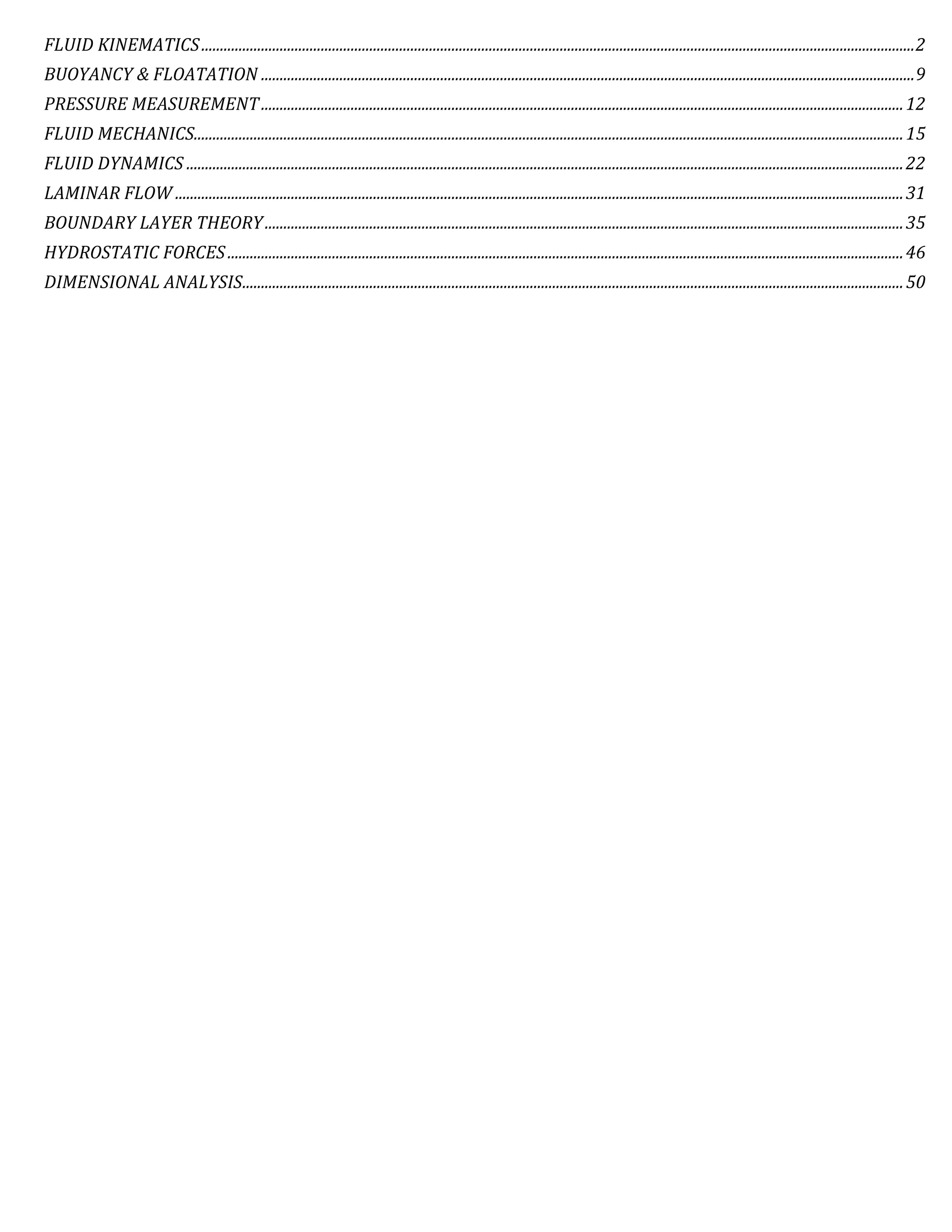
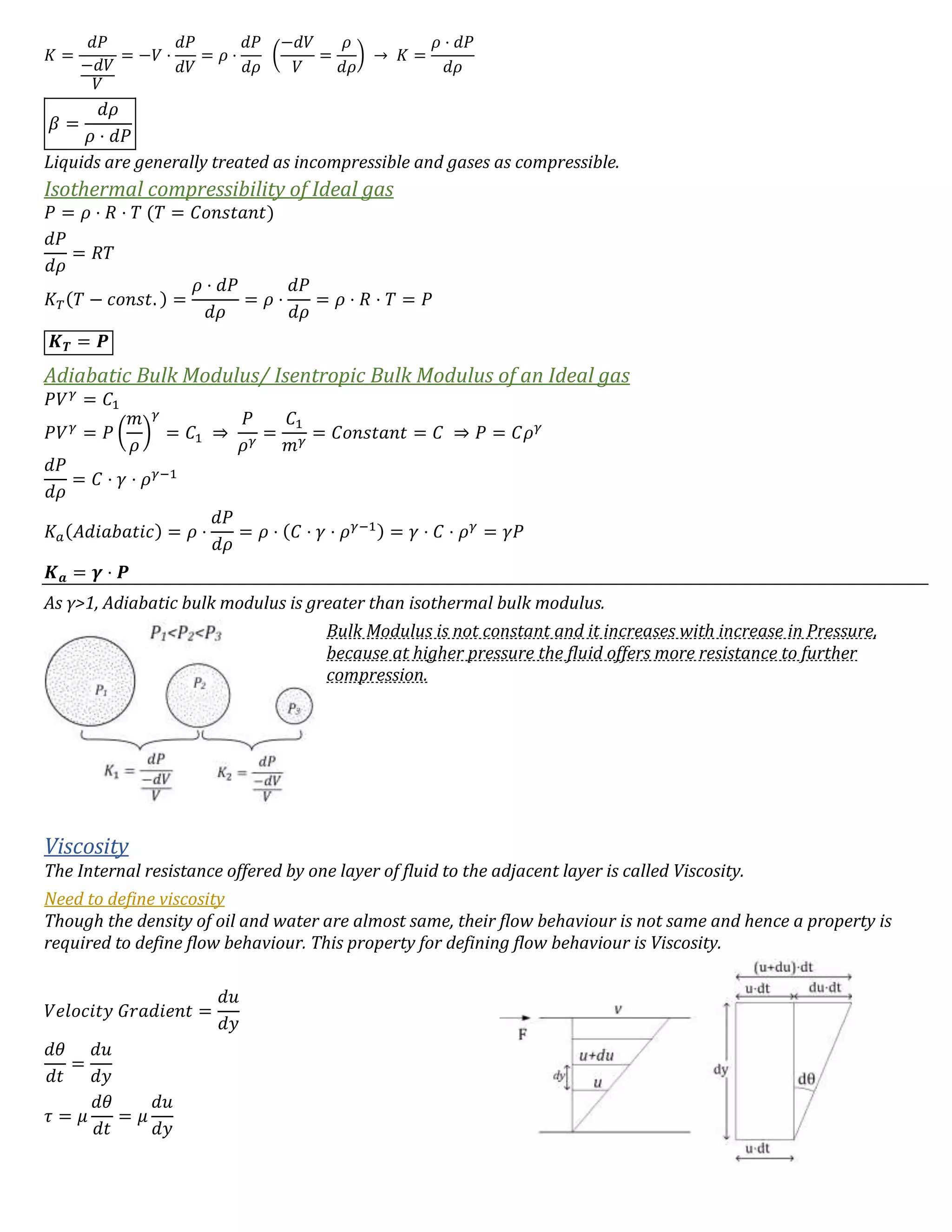
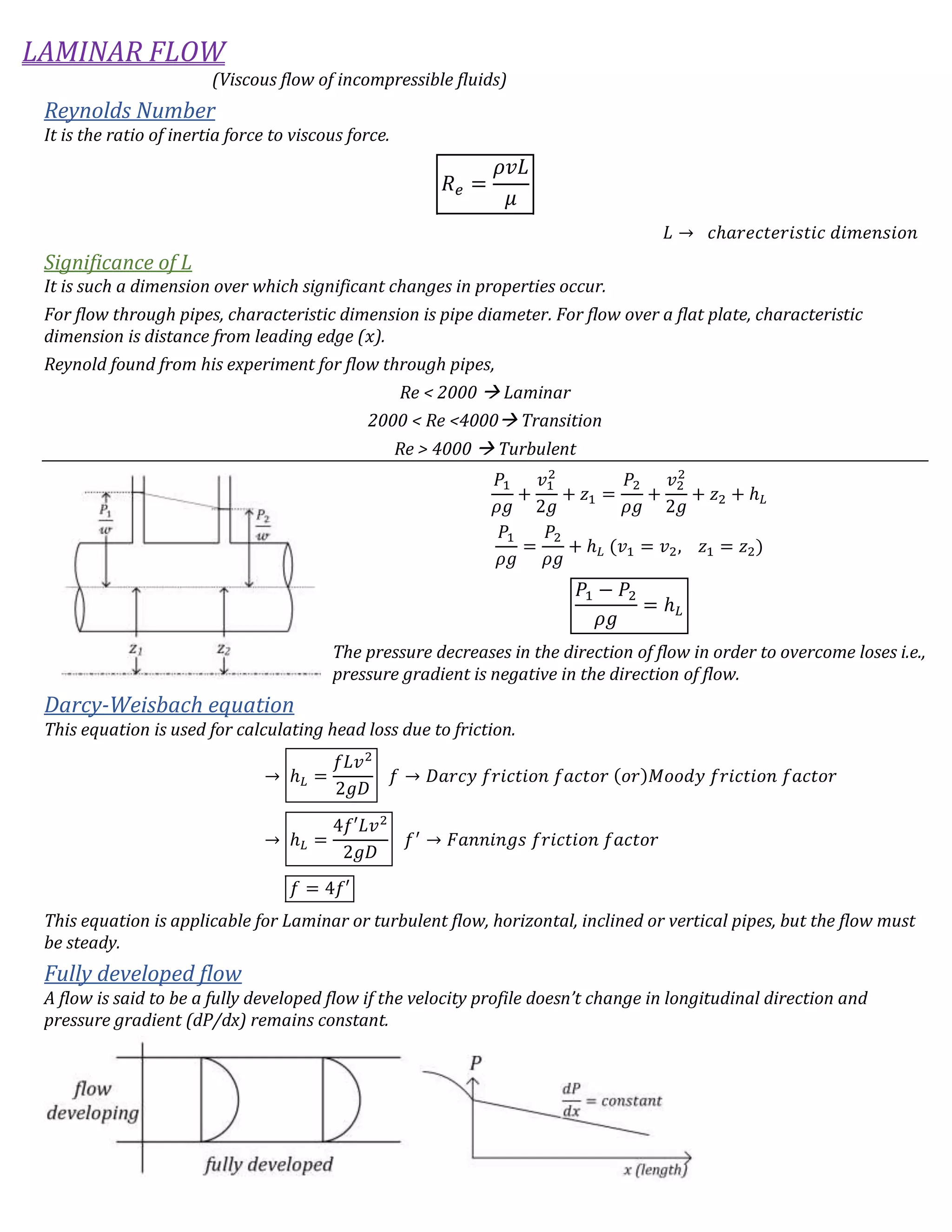
![Circulation (Γ)
It is the line integral of tangential component of velocity taken
around a closed curve.
𝛤 = 𝑢 ⋅ 𝑑𝑥 + (𝑣 +
𝜕𝑣
𝜕𝑥
𝑑𝑥) ⋅ 𝑑𝑦 − (𝑢 +
𝜕𝑢
𝜕𝑦
𝑑𝑦) ⋅ 𝑑𝑥 − 𝑣 ⋅ 𝑑𝑦
𝛤 = (
𝜕𝑣
𝜕𝑥
−
𝜕𝑢
𝜕𝑦
) 𝑑𝑥 ⋅ 𝑑𝑦
[𝐴𝑟𝑒𝑎 = 𝑑𝑥 ⋅ 𝑑𝑦]
𝐶𝑖𝑟𝑐𝑢𝑙𝑎𝑡𝑖𝑜𝑛 (𝛤) = 𝑉𝑜𝑟𝑡𝑖𝑐𝑖𝑡𝑦 (2𝜔 𝑧) × 𝐴𝑟𝑒𝑎
In case of irrotational flow, vorticity is zero & circulation is zero.
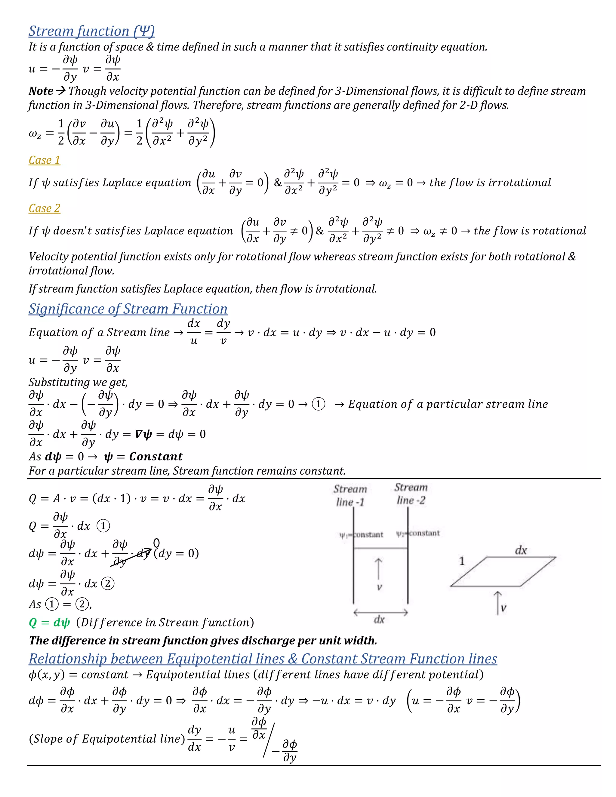
Velocity Potential function (ϕ)
It is a function of space & time defined in such a manner, that its negative derivative w.r.t space gives velocity in
that direction. The negative sign is taken as the flow is in the direction of decreasing potential.
−
𝜕𝜙
𝜕𝑥
= 𝑢 −
𝜕𝜙
𝜕𝑦
= 𝑣 −
𝜕𝜙
𝜕𝑧
= 𝑤
Velocity potential function can be defined for 2-Dimensional flow
𝜕𝑢
𝜕𝑥
+
𝜕𝑣
𝜕𝑥
=
𝜕
𝜕𝑥
(−
𝜕𝜙
𝜕𝑥
) +
𝜕
𝜕𝑦
(−
𝜕𝜙
𝜕𝑦
) = − (
𝜕2
𝜙
𝜕𝑥2
+
𝜕2
𝜙
𝜕𝑦2
)
Case 1
𝐼𝑓
𝜕2
𝜙
𝜕𝑥2
+
𝜕2
𝜙
𝜕𝑦2
= 0, 𝝓 𝒔𝒂𝒕𝒊𝒔𝒇𝒊𝒆𝒔 𝑳𝒂𝒑𝒍𝒂𝒄𝒆 𝒆𝒒𝒖𝒂𝒕𝒊𝒐𝒏 𝑎𝑠 (
𝜕𝑢
𝜕𝑥
+
𝜕𝑣
𝜕𝑥
= 0)
→ Continuity equation is satisfied and flow is possible.
Case 2
𝐼𝑓
𝜕2
𝜙
𝜕𝑥2
+
𝜕2
𝜙
𝜕𝑦2
≠ 0, 𝝓 𝒅𝒐𝒆𝒔𝒏′
𝒕 𝒔𝒂𝒕𝒊𝒔𝒇𝒊𝒆𝒔 𝑳𝒂𝒑𝒍𝒂𝒄𝒆 𝒆𝒒𝒖𝒂𝒕𝒊𝒐𝒏 𝑎𝑠 (
𝜕𝑢
𝜕𝑥
+
𝜕𝑣
𝜕𝑥
≠ 0)
→ Continuity equation is not satisfied and flow is not possible.
Case 3
𝜔 𝑧 =
1
2
(
𝜕𝑣
𝜕𝑥
−
𝜕𝑢
𝜕𝑦
) =
1
2
(−
𝜕2
𝜙
𝜕𝑥 ⋅ 𝜕𝑦
+
𝜕2
𝜙
𝜕𝑦 ⋅ 𝜕𝑥
)
𝜔 𝑧 = 0 → 𝐼𝑟𝑟𝑜𝑡𝑎𝑡𝑖𝑜𝑛𝑎𝑙 𝑓𝑙𝑜𝑤
Velocity Potential function exits only for Irrotational flow i.e., the existence of velocity potential function
implies the flow is irrotational. Sometimes irrotational flow are also known as Potential flow.](https://image.slidesharecdn.com/fluidmechanicsfinal-180307190704/75/Fluid-mechanics-notes-for-gate-8-2048.jpg)
![𝑢 =
1
4𝜇
(
𝜕𝑃
𝜕𝑥
) ⋅ 𝑟2
−
1
4𝜇
(
𝜕𝑃
𝜕𝑥
) ⋅ 𝑅2
𝑢 = −
1
4𝜇
(
𝜕𝑃
𝜕𝑥
) [𝑅2
− 𝑟2]
(𝑙𝑜𝑐𝑎𝑙 𝑣𝑒𝑙𝑜𝑐𝑖𝑡𝑦)𝑢 = −
1
4𝜇
(
𝜕𝑃
𝜕𝑥
) ⋅ 𝑅2
⋅ [1 −
𝑟2
𝑅2
]
𝑊𝑒 𝑔𝑒𝑡 𝑢 𝑚𝑎𝑥 𝑤ℎ𝑒𝑛 𝑟 = 0,
𝑢 𝑚𝑎𝑥 = −
1
4𝜇
(
𝜕𝑃
𝜕𝑥
) ⋅ 𝑅2
𝑢 = 𝑢 𝑚𝑎𝑥 ⋅ [1 −
𝑟2
𝑅2
]
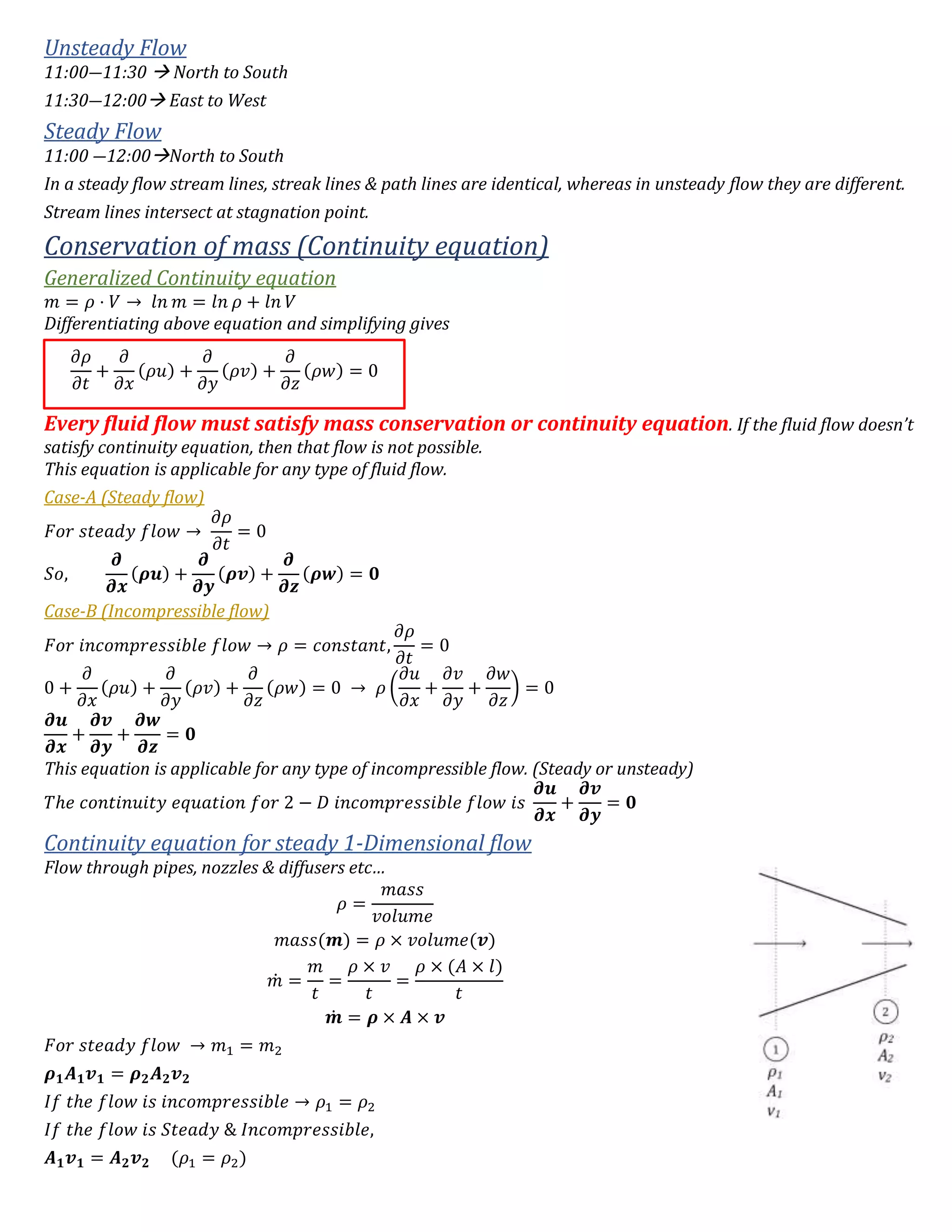
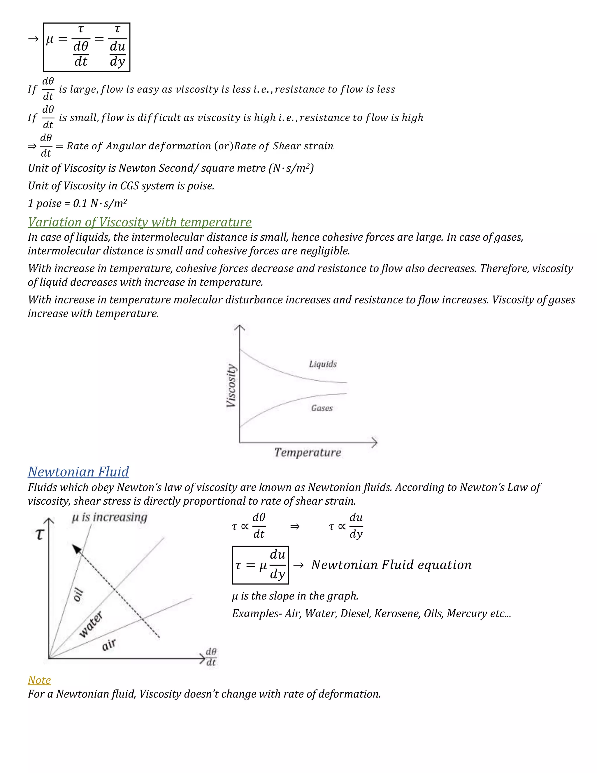
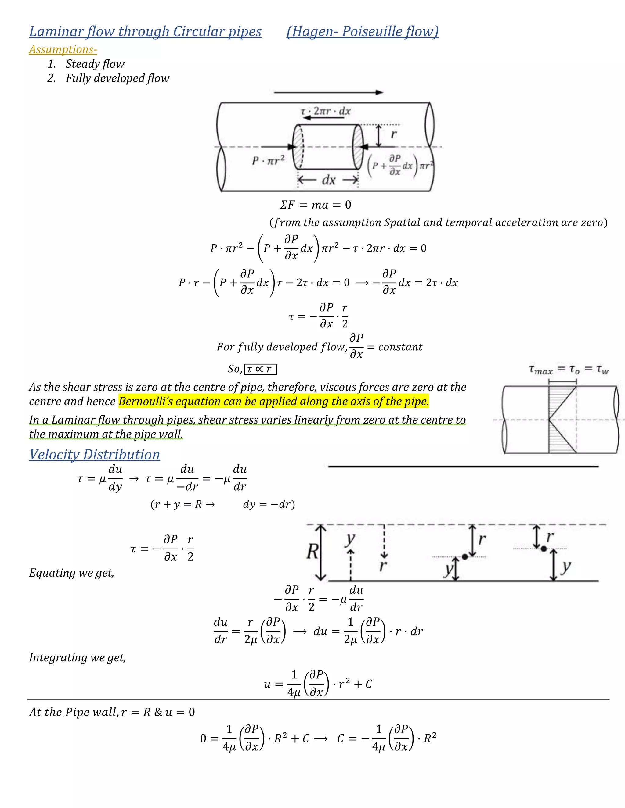
The velocity distribution is parabolic in Laminar flow through pipes.
Discharge
Let us calculate discharge through elemental ring,
𝑑𝑄 = 𝑢 ⋅ 2𝜋𝑟 ⋅ 𝑑𝑟
𝑄 = ∫ 𝑢 ⋅ 2𝜋𝑟 ⋅ 𝑑𝑟
𝑅
0
= ∫ 𝑢 𝑚𝑎𝑥 ⋅ [1 −
𝑟2
𝑅2
] ⋅ 2𝜋𝑟 ⋅ 𝑑𝑟
𝑅
0
= 2𝜋 ⋅ 𝑢 𝑚𝑎𝑥 [
𝑟2
2
−
𝑟4
4𝑅2
]
0
𝑅
𝑄 = 2𝜋 ⋅ 𝑢 𝑚𝑎𝑥 [
𝑅2
2
−
𝑅2
4
] = 2𝜋 ⋅ 𝑢 𝑚𝑎𝑥 ⋅
𝑅2
4
𝑄 =
𝑢 𝑚𝑎𝑥 ⋅ 𝜋𝑅2
2
𝑄 =
𝜋 ⋅ 𝑢 𝑚𝑎𝑥 ⋅ 𝑅2
2
=
𝜋 ⋅ 𝑅2
2
(−
1
4𝜇
(
𝜕𝑃
𝜕𝑥
) ⋅ 𝑅2
)
𝑄 = −
𝜋
8𝜇
(
𝜕𝑃
𝜕𝑥
) ⋅ 𝑅4](https://image.slidesharecdn.com/fluidmechanicsfinal-180307190704/75/Fluid-mechanics-notes-for-gate-34-2048.jpg)
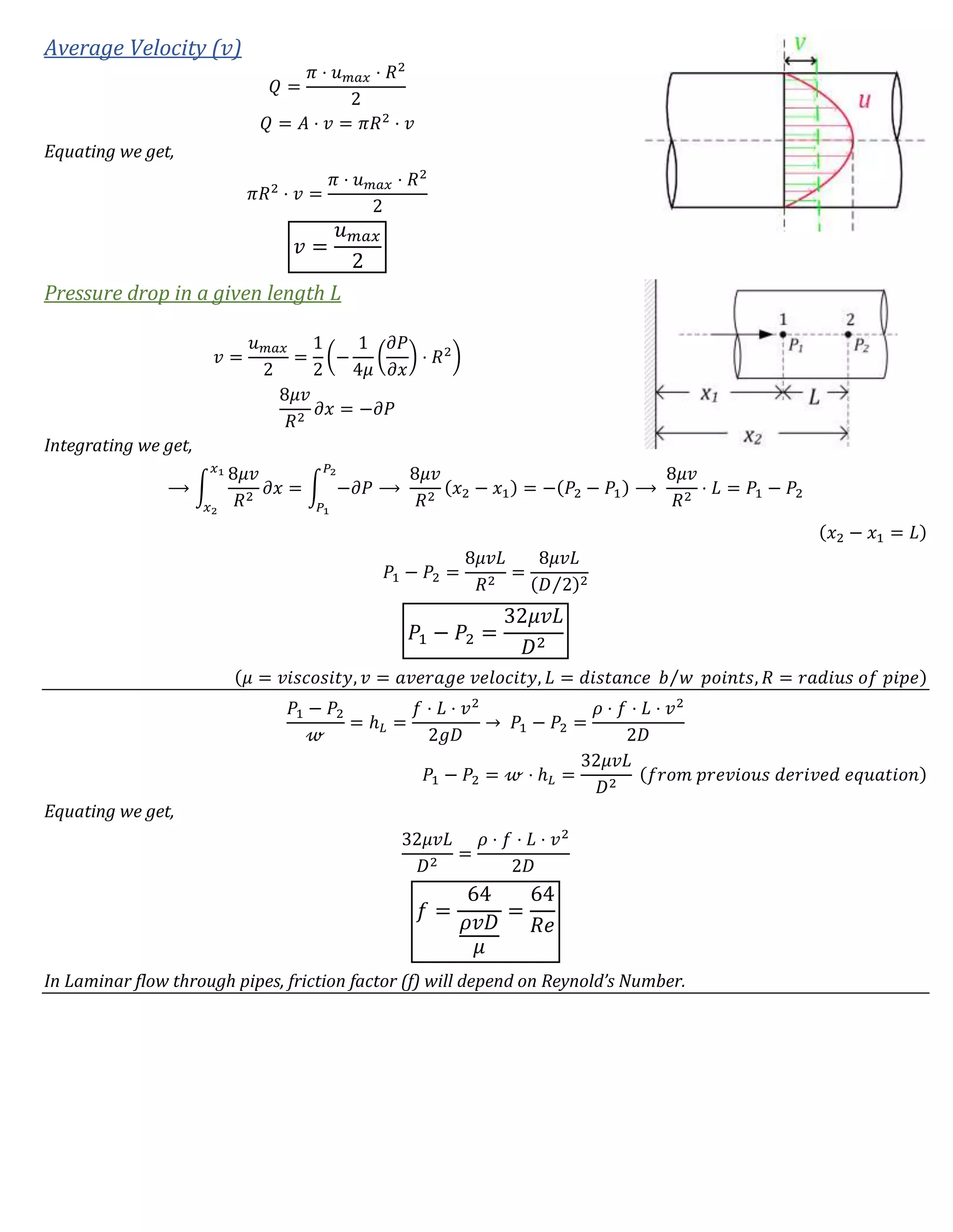
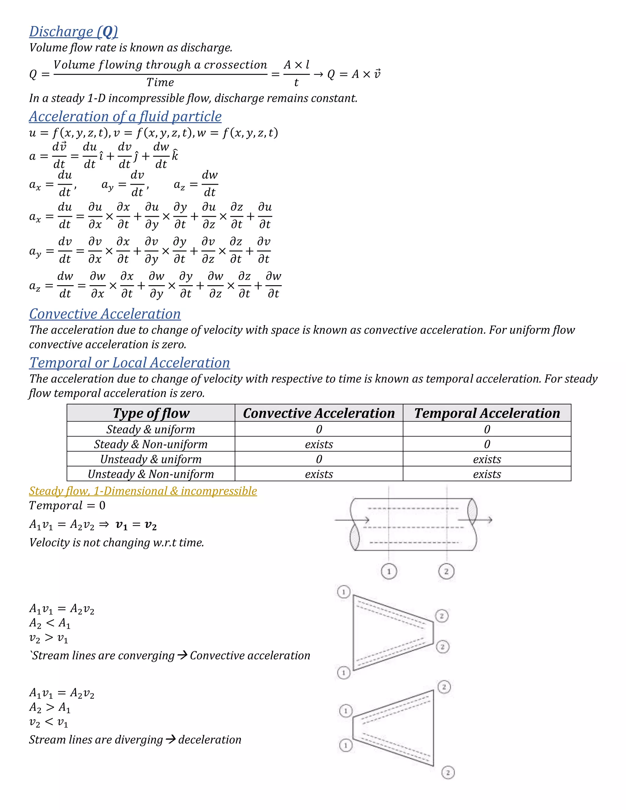
![Buckingham’s pi theorem
If there are n no. of total variables, and m no. of fundamental quantities, then given systems can be grouped into
n-m pi terms.
The resistance force F of a ship is a function of length ‘l’, velocity ‘v’, acceleration due to gravity ‘g’ and fluid
properties like density ‘ρ’, viscosity ‘μ’, and write the relationship in dimensionless form using buckingham’s pi
theorem.
𝐹 = 𝜙(𝐿, 𝑣, 𝑔, 𝜌, 𝜇)
𝑛 = 6, 𝑚 = 3
[𝐹 → 𝑀𝐿𝑇−2
, 𝑔 → 𝐿𝑇−2
, 𝜌 → 𝐿−3
, 𝜇 → 𝑀𝐿−1
𝑇−1
, 𝑣 → 𝐿𝑇−1]
𝑇ℎ𝑒 𝑔𝑖𝑣𝑒𝑛 𝑠𝑦𝑠𝑡𝑒𝑚 𝑣𝑎𝑛 𝑏𝑒 𝑔𝑟𝑜𝑢𝑝𝑒𝑑 𝑖𝑛𝑡𝑜 6 − 3 = 3, 3 𝜋 𝑡𝑒𝑟𝑚𝑠
Selection of repeated variables
1. Repeated variables must be selected from independent variables.
2. Number of repeated variables is equal to number of fundamental quantities.
3. Each repeated variable must have its own dimension.
4. Repeated variable group must contain all fundamental quantities.
5. Most fundamental quantity must be selected as repeated variable.
→ 𝐹 = 𝜙(𝐿, 𝑣, 𝑔, 𝜌, 𝜇)
→ 𝜋1 = 𝐹 ⋅ 𝐿 𝑎1
⋅ 𝑣 𝑏1
⋅ 𝜌 𝑐1
→ 𝜋2 = 𝑔 ⋅ 𝐿 𝑎2
⋅ 𝑣 𝑏2
⋅ 𝜌 𝑐2
→ 𝜋3 = 𝜇 ⋅ 𝐿 𝑎3
⋅ 𝑣 𝑏3
⋅ 𝜌 𝑐3
𝝅 𝟏 →
𝑀0
𝐿0
𝑇0
= 𝑀𝐿𝑇−2
⋅ 𝐿 𝑎1
⋅ (𝐿𝑇−1) 𝑏1
⋅ (𝑀𝐿−3) 𝑐1
𝑀0
𝐿0
𝑇0
= 𝑀1+𝑐1 ⋅ 𝐿1+𝑎1+𝑏1−3𝑐1 ⋅ 𝑇−2−𝑏1
𝑐1 = −1 𝑏1 = −2 𝑎1 = −2
𝜋1 =
𝐹
𝐿2 𝑣2 𝜌
𝑆𝑖𝑚𝑖𝑙𝑎𝑟𝑙𝑦, 𝜋2 =
𝑔𝐿
𝑣2
𝜋3 =
𝜇
𝜌𝑣𝐿
→ 𝐹 = 𝜙(𝐿, 𝑣, 𝑔, 𝜌, 𝜇)
→ 𝜋1 = 𝜙(𝜋2, 𝜋3) →
𝐹
𝐿2 𝑣2 𝜌
= 𝜙 (
𝑔𝐿
𝑣2
,
𝜇
𝜌𝑣𝐿
) → 𝐹 = 𝜌𝐿2
𝑣2
⋅ 𝜙 (
𝑔𝐿
𝑣2
,
𝜇
𝜌𝑣𝐿
)
Various forces in fluid mechanics
Inertia force
𝐹𝑖 = 𝑚 ⋅ 𝑎
[𝜌 =
𝑚
𝑉3
=
𝑚
𝐿3
→ 𝑚 = 𝜌 ⋅ 𝐿3
, 𝑎 =
𝑣
𝑇
]
𝐹𝑖 = 𝜌 ⋅ 𝐿3
⋅
𝑣
𝑇
= 𝜌 ⋅ 𝐿2
⋅
𝐿
𝑇
⋅ 𝑣 → 𝐹𝑖 = 𝜌 ⋅ 𝐿2
⋅ 𝑣2
Pressure Force
𝑃 =
𝐹𝑃
𝐴
→ 𝐹𝑃 = 𝑃 ⋅ 𝐴
𝐹𝑃 = 𝑃 ⋅ 𝐿2](https://image.slidesharecdn.com/fluidmechanicsfinal-180307190704/75/Fluid-mechanics-notes-for-gate-52-2048.jpg)
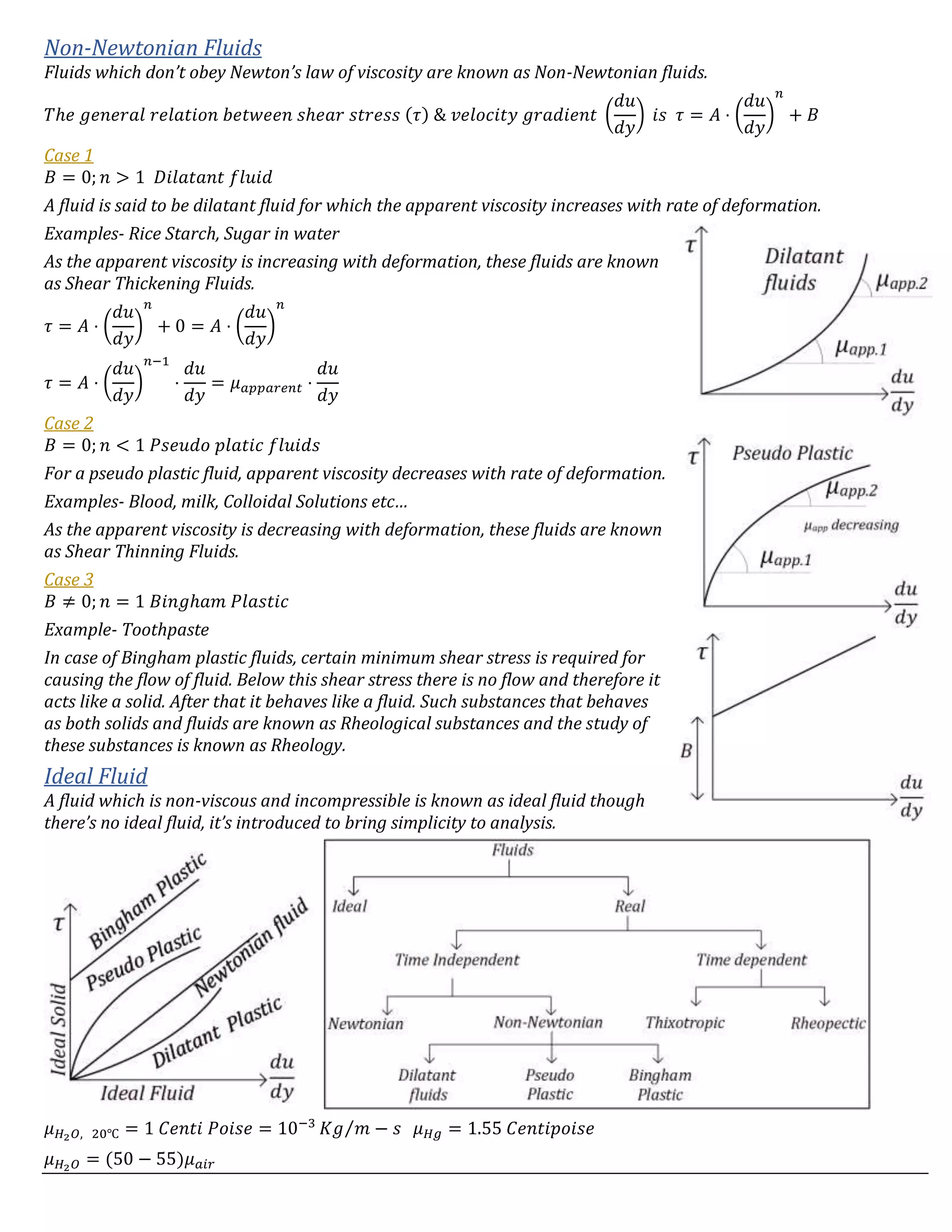
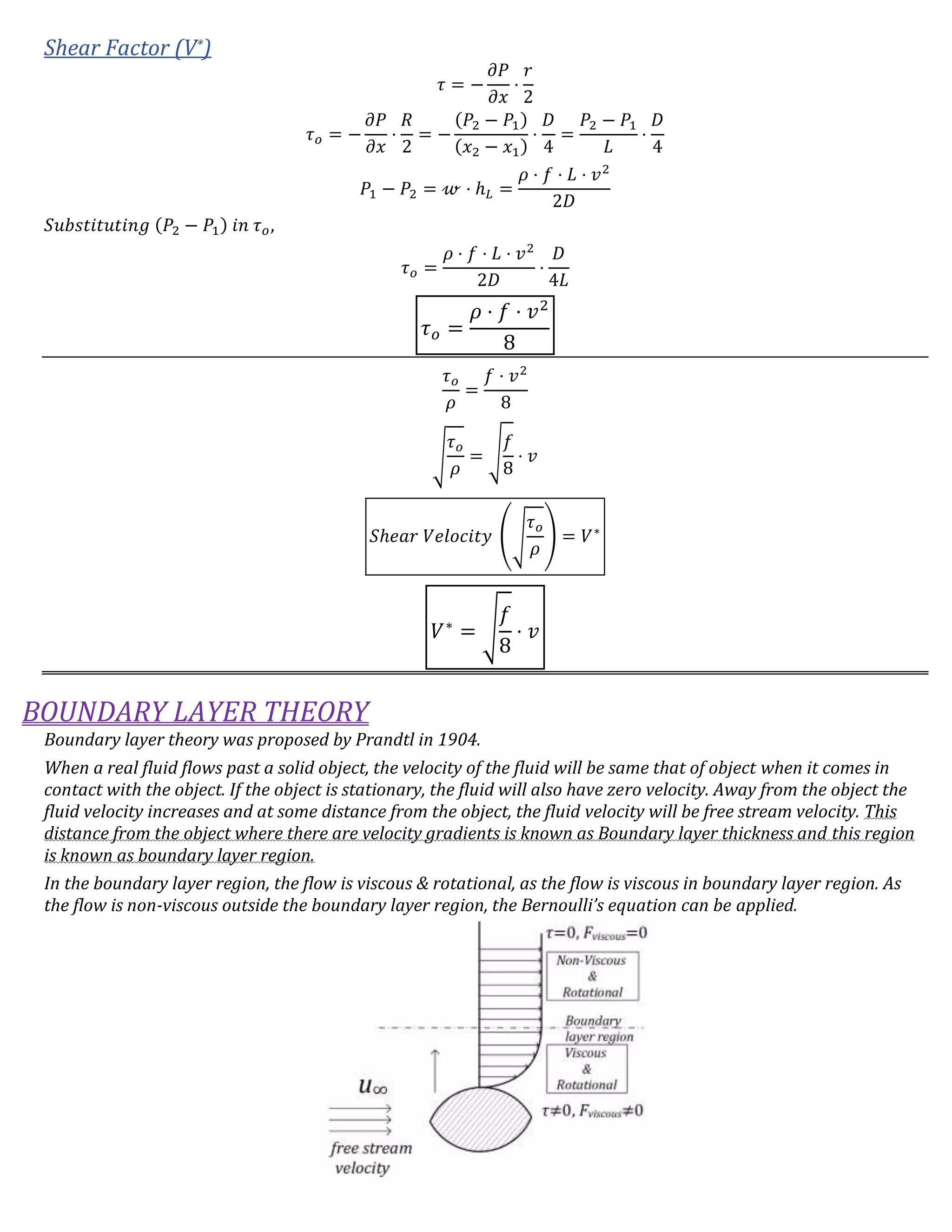
![Gravity force
𝐹𝑔 = 𝑚𝑔
𝐹𝑔 = 𝜌 ⋅ 𝐿3
⋅ 𝑔 [𝑚 = 𝜌 ⋅ 𝐿3]
Surface tension force
𝜎 =
𝐹𝑠
𝐿
𝐹𝑠 = 𝜎 ⋅ 𝐿
Viscous force
𝐹𝑣 =
𝜇 ⋅ 𝐴 ⋅ 𝑣
𝑦
𝐹𝑣 =
𝜇 ⋅ 𝐿2
⋅ 𝑣
𝐿
𝐹𝑣 = 𝜇 ⋅ 𝐿 ⋅ 𝑣
Elastic force
When a fluid is compresses, there is a rise in pressure, this rise in pressure is proportional to bulk modulus and this
rise in pressure gives rise to a force known as elastic force.
𝐹𝑒 = 𝐾 ⋅ 𝐿2
Various dimensionless numbers in fluid mechanics
Reynold’s number
It’s defined as the ratio of inertia force to viscous force.
→ 𝑅𝑒 =
𝐹𝑖
𝐹𝑣
=
𝜌 ⋅ 𝐿2
⋅ 𝑣2
𝜇 ⋅ 𝐿 ⋅ 𝑣
=
𝜌 ⋅ 𝐿 ⋅ 𝑣
𝜇
→ 𝑅𝑒 =
𝜌 ⋅ 𝐿 ⋅ 𝑣
𝜇
Euler number
𝐸𝑢 =
𝐹𝑖
𝐹𝑃
=
𝜌 ⋅ 𝐿2
⋅ 𝑣2
𝑃 ⋅ 𝐿2
𝐸𝑢 =
𝜌 ⋅ 𝑣2
𝑃
Froude number
𝐹𝑟 =
𝐹𝑖
𝐹𝑔
=
𝜌 ⋅ 𝐿2
⋅ 𝑣2
𝜌 ⋅ 𝐿3 ⋅ 𝑔
𝐹𝑟 =
𝑣2
𝑔 ⋅ 𝐿
Weber number
It’s the ratio of inertia force to surface tension force.
𝑊𝑒 =
𝐹𝑖
𝐹𝑠
=
𝜌 ⋅ 𝐿 ⋅ 𝑣2
𝜎 ⋅ 𝐿
𝑊𝑒 =
𝜌 ⋅ 𝑣2
𝜎](https://image.slidesharecdn.com/fluidmechanicsfinal-180307190704/75/Fluid-mechanics-notes-for-gate-53-2048.jpg)

The document discusses key concepts in fluid mechanics including: 1. Fluid kinematics deals with fluid motion without reference to forces, using Lagrangian and Eulerian techniques. Different types of flow include steady/unsteady, uniform/non-uniform, and laminar/turbulent. 2. Streamlines, pathlines, and streaklines are defined. Streamlines give the instantaneous flow pattern. Continuity equations are derived for compressible, incompressible, 1D, and 2D steady flows. 3. Discharge is defined as the volume flow rate through a cross-section. Acceleration terms including convective and temporal acceleration are explained for different flow types.
Introduction to fluid mechanics covering various topics such as fluid kinematics, dynamics, and other foundational concepts.
Fluid kinematics addresses the motion of fluids, outlining techniques like Lagrangian and Eulerian approaches, and distinguishes flow types including steady, unsteady, laminar, and turbulent.
Discusses the continuity equation for mass conservation in fluid flow, illustrating steady and unsteady, as well as incompressible flow dynamics.
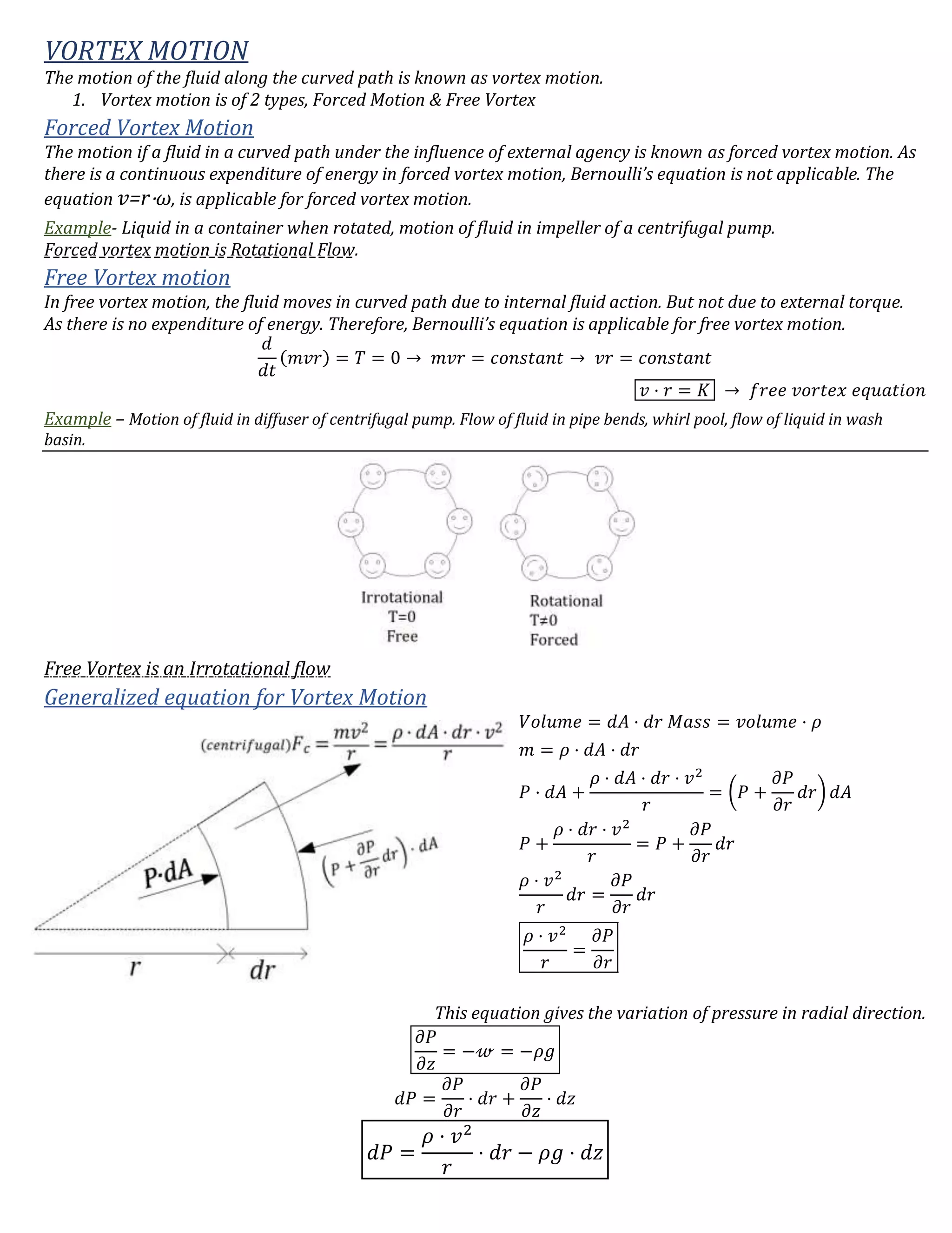
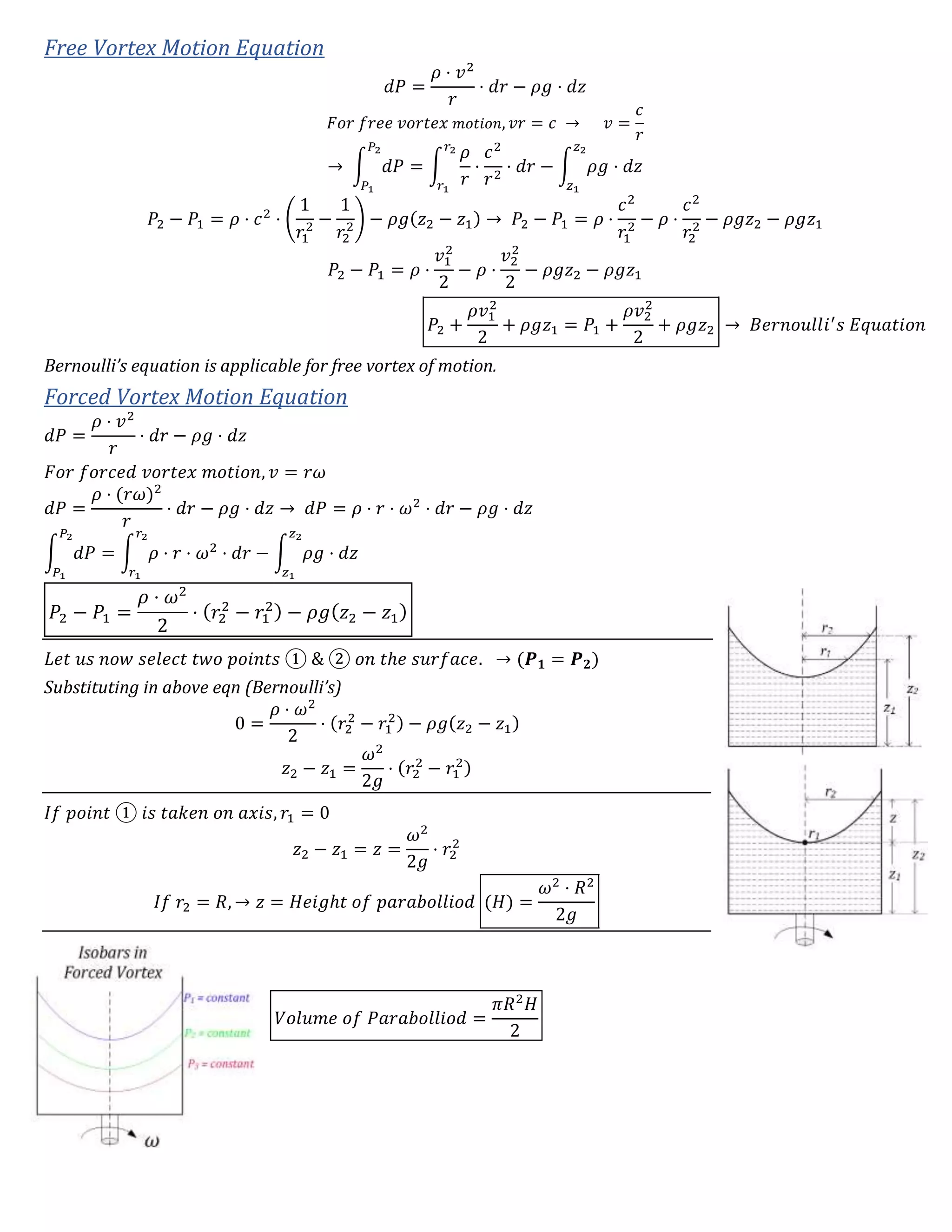
Examines angular velocity, vorticity, circulation, and defines conditions for rotational and irrotational flow types.
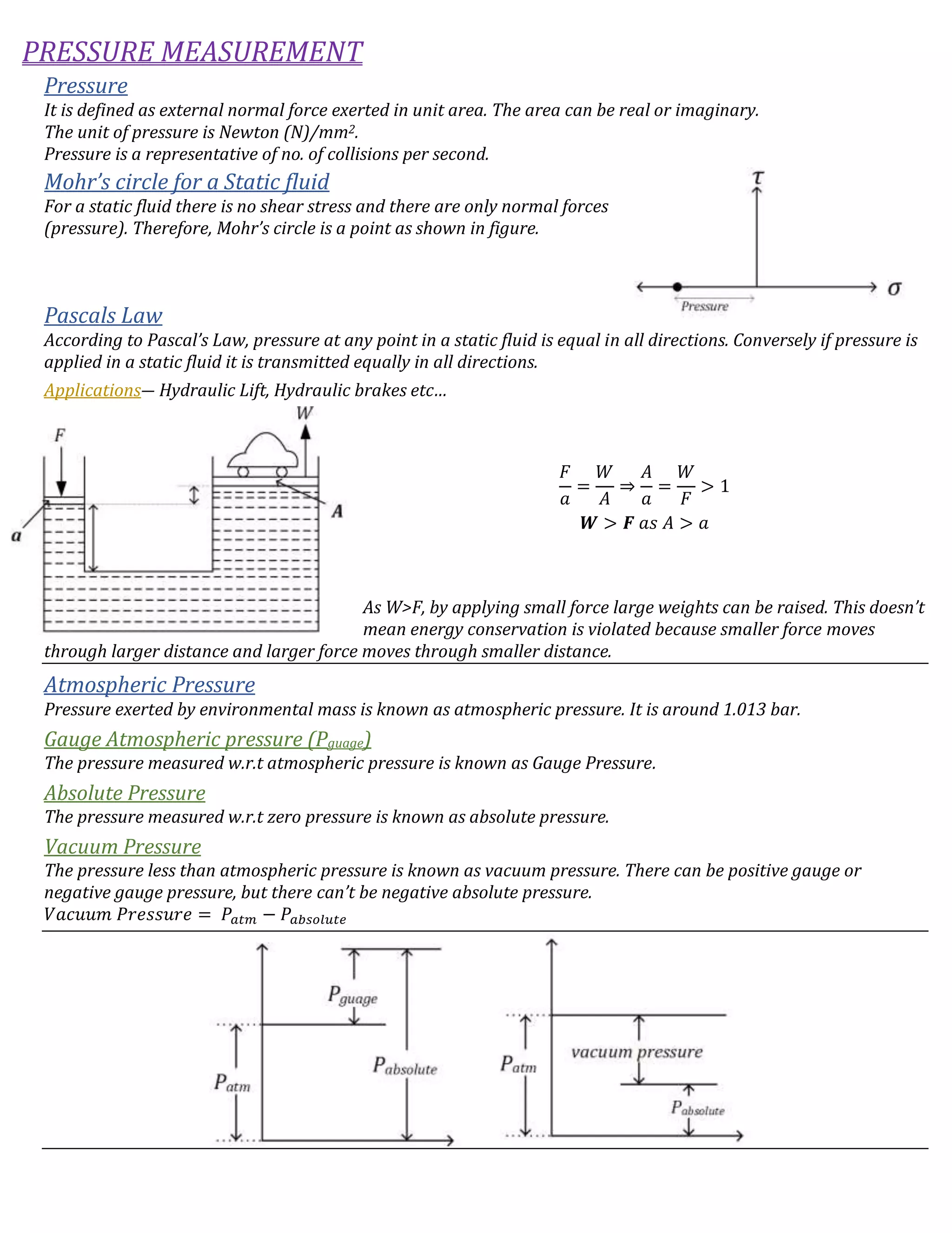
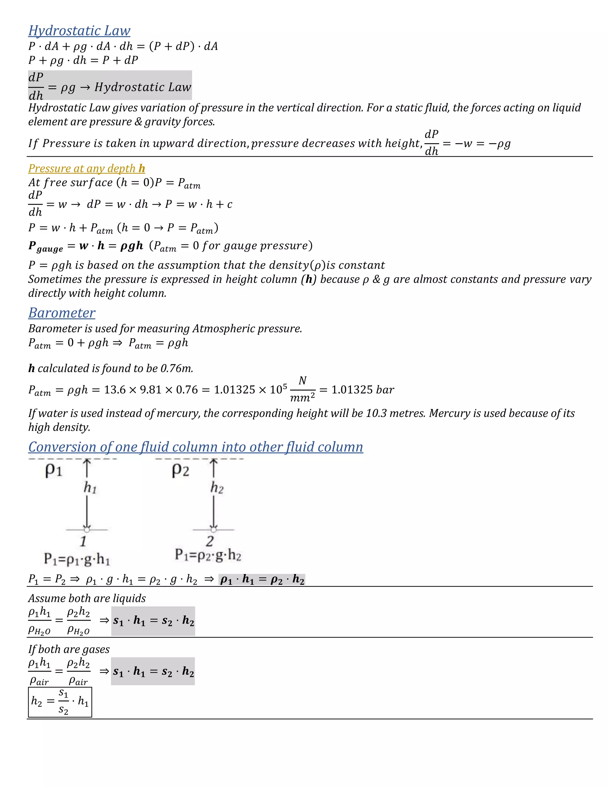
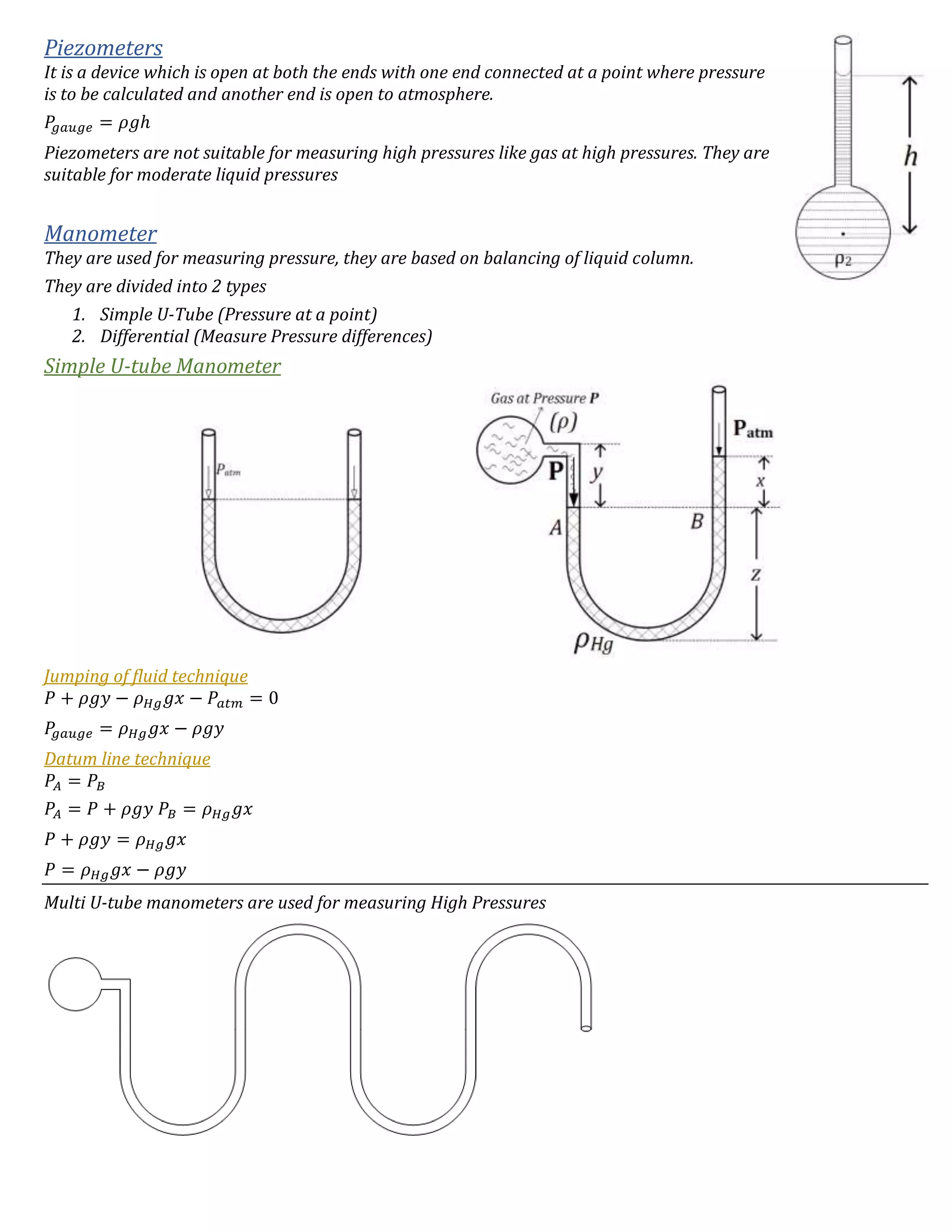
Defines pressure, hydrostatic law, various pressure types, including absolute and gauge pressure, and introduces measurement devices like piezometers and manometers.
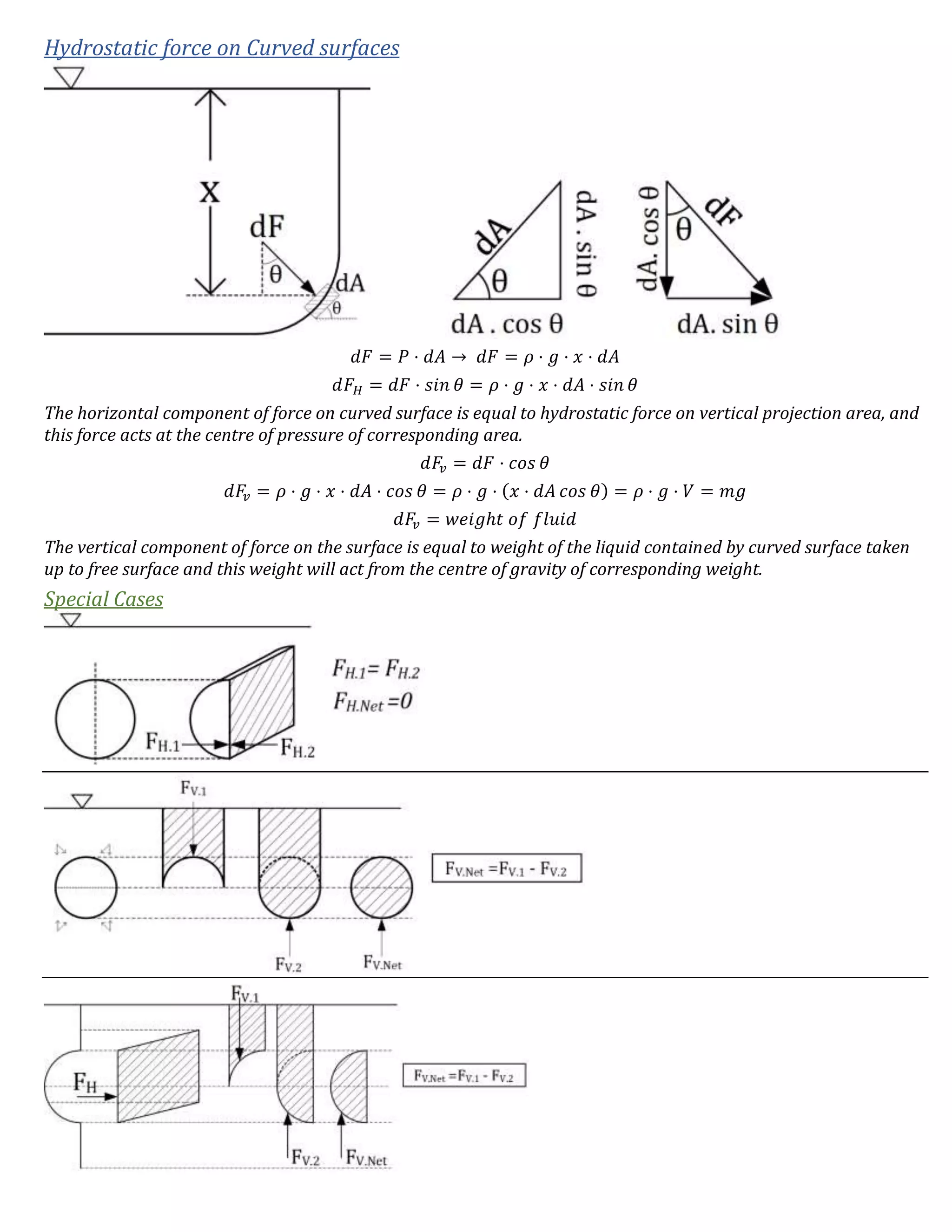
Describes hydrostatic fluid properties, distinctions between fluids and solids, and hydrostatic forces on surfaces with relevant equations.
Defines viscosity, differentiates between Newtonian and Non-Newtonian fluids, and examines how temperature affects fluid viscosity.
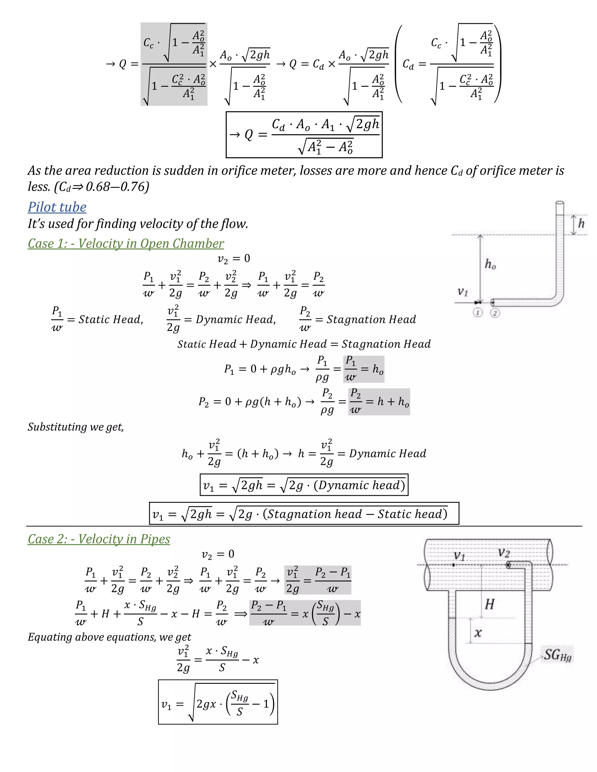
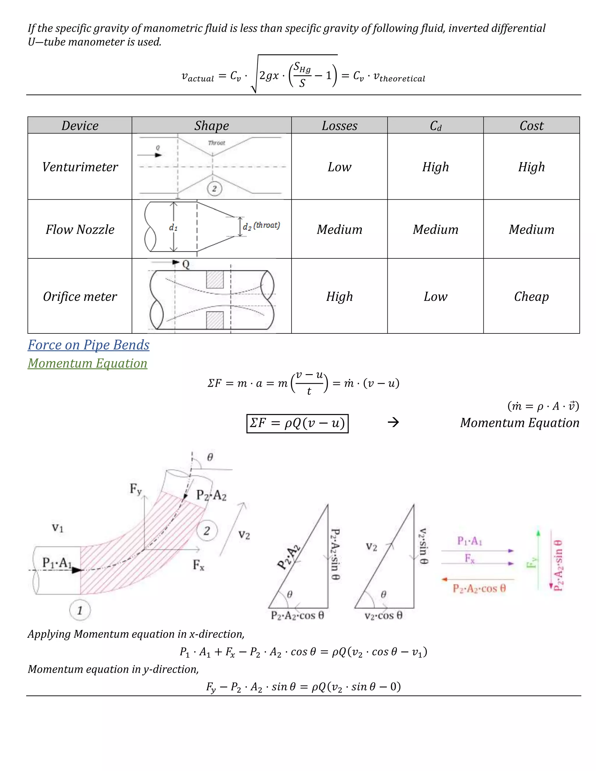
Examines practical applications of fluid dynamics, including the Venturimeter, Orifice meters, and discussion on various fluid flow equations.
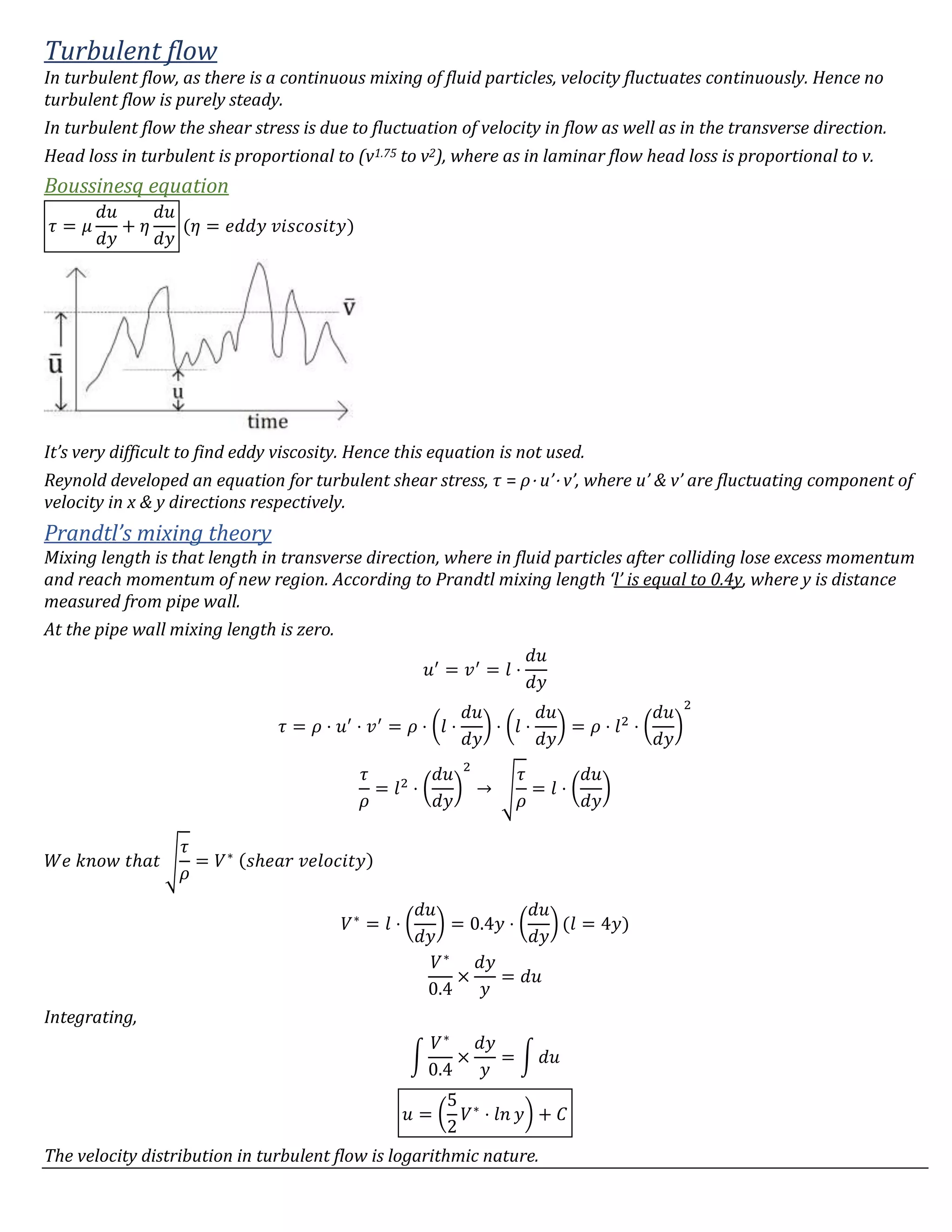
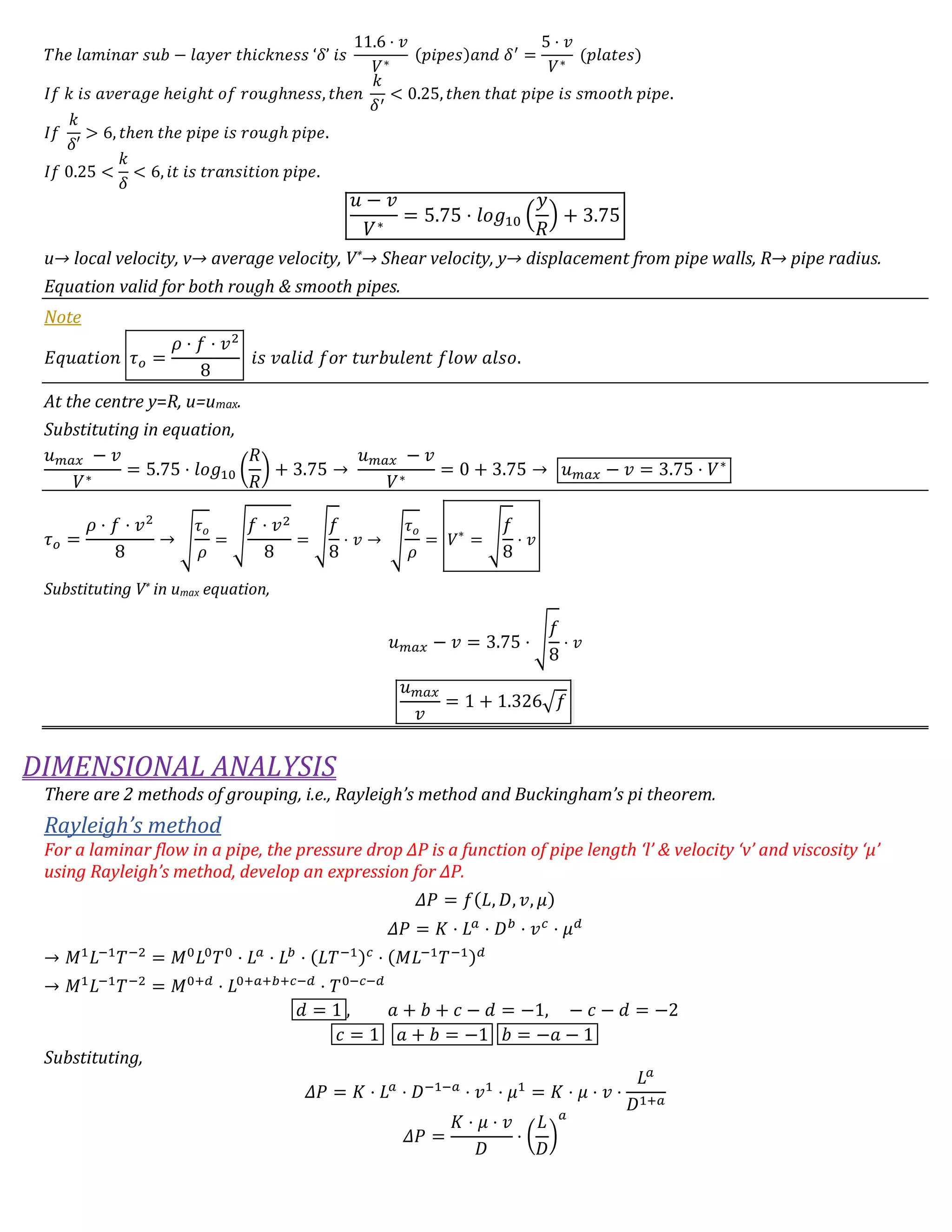
Detail on turbulent flow characteristics, shear stress equations, and different forces acting on fluids including inertial and gravitational forces. Presents dimensional analysis methods such as Rayleigh's method and Buckingham's pi theorem for deriving relationships in fluid mechanics.


