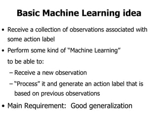
This machine learning foundations course will consist of 4 homework assignments, both theoretical and programming problems in Matlab. There will be a final exam. Students will work in groups of 2-3 to take notes during classes in LaTeX format. These class notes will contribute 30% to the overall grade. The course will cover basic machine learning concepts like storage and retrieval, learning rules, estimating flexible models, and applications in areas like control, medical diagnosis, and document retrieval.

1. Machine Learning : Foundations Course Number 0368403401 Prof. Nathan Intrator TA: Daniel Gill, Guy Amit

2. Course structure There will be 4 homework exercises They will be theoretical as well as programming All programming will be done in Matlab Course info accessed from www.cs.tau.ac.il/~nin Final has not been decided yet Office hours Wednesday 4-5 (Contact via email)

3. Class Notes Groups of 2-3 students will be responsible for a scribing class notes Submission of class notes by next Monday (1 week) and then corrections and additions from Thursday to the following Monday 30% contribution to the grade

4. Class Notes (cont) Notes will be done in LaTeX to be compiled into PDF via miktex. (Download from School site) Style file to be found on course web site Figures in GIF

5. Basic Machine Learning idea Receive a collection of observations associated with some action label Perform some kind of “Machine Learning” to be able to: Receive a new observation “ Process” it and generate an action label that is based on previous observations Main Requirement: Good generalization

6. Learning Approaches Store observations in memory and retrieve Simple, little generalization (Distance measure?) Learn a set of rules and apply to new data Sometimes difficult to find a good model Good generalization Estimate a “flexible model” from the data Generalization issues, data size issues

7. Storage & Retrieval Simple, computationally intensive little generalization How can retrieval be performed? Requires a “distance measure” between stored observations and new observation Distance measure can be given or “learned” (Clustering)

8. Learning Set of Rules How to create “reliable” set of rules from the observed data Tree structures Graphical models Complexity of the set of rules vs. generalization

9. Estimation of a flexible model What is a “flexible” model Universal approximator Reliability and generalization, Data size issues

10. Applications Control Robot arm Driving and navigating a car Medical applications: Diagnosis, monitoring, drug release Web retrieval based on user profile Customized ads: Amazon Document retrieval: Google

11. Related Disciplines machine learning AI probability & statistics computational complexity theory control theory information theory philosophy psychology neurophysiology ethology decision theory game theory optimization biological evolution statistical mechanics

12. Why Now? Technology ready: Algorithms and theory. Information abundant: Flood of data (online) Computational power Sophisticated techniques Industry and consumer needs.

13. Example 1: Credit Risk Analysis Typical customer: bank. Database: Current clients data, including: basic profile (income, house ownership, delinquent account, etc.) Basic classification. Goal: predict/decide whether to grant credit.

14. Example 1: Credit Risk Analysis Rules learned from data: IF Other-Delinquent-Accounts > 2 and Number-Delinquent-Billing-Cycles >1 THEN DENAY CREDIT IF Other-Delinquent-Accounts = 0 and Income > $30k THEN GRANT CREDIT

15. Example 2: Clustering news Data: Reuters news / Web data Goal: Basic category classification: Business, sports, politics, etc. classify to subcategories (unspecified) Methodology: consider “typical words” for each category. Classify using a “distance “ measure.

16. Example 3: Robot control Goal: Control a robot in an unknown environment. Needs both to explore (new places and action) to use acquired knowledge to gain benefits. Learning task “control” what is observes!

18. History of Machine Learning (cont’d) 1960’s and 70’s: Models of human learning High-level symbolic descriptions of knowledge, e.g., logical expressions or graphs/networks, e.g., (Karpinski & Michalski, 1966) (Simon & Lea, 1974). META-DENDRAL (Buchanan, 1978), for example, acquired task-specific expertise (for mass spectrometry) in the context of an expert system. Winston’s (1975) structural learning system learned logic-based structural descriptions from examples. 1970’s: Genetic algorithms Developed by Holland (1975) 1970’s - present: Knowledge-intensive learning A tabula rasa approach typically fares poorly. “To acquire new knowledge a system must already possess a great deal of initial knowledge.” Lenat’s CYC project is a good example.

19. History of Machine Learning (cont’d) 1970’s - present: Alternative modes of learning (besides examples) Learning from instruction, e.g., (Mostow, 1983) (Gordon & Subramanian, 1993) Learning by analogy, e.g., (Veloso, 1990) Learning from cases, e.g., (Aha, 1991) Discovery (Lenat, 1977) 1991: The first of a series of workshops on Multistrategy Learning (Michalski) 1970’s – present: Meta-learning Heuristics for focusing attention, e.g., (Gordon & Subramanian, 1996) Active selection of examples for learning, e.g., (Angluin, 1987), (Gasarch & Smith, 1988), (Gordon, 1991) Learning how to learn, e.g., (Schmidhuber, 1996)

20. History of Machine Learning (cont’d) 1980 – The First Machine Learning Workshop was held at Carnegie-Mellon University in Pittsburgh. 1980 – Three consecutive issues of the International Journal of Policy Analysis and Information Systems were specially devoted to machine learning. 1981 – A special issue of SIGART Newsletter reviewed current projects in the field of machine learning. 1983 – The Second International Workshop on Machine Learning, in Monticello at the University of Illinois. 1986 – The establishment of the Machine Learning journal. 1987 – The beginning of annual international conferences on machine learning (ICML). 1988 – The beginning of regular workshops on computational learning theory (COLT). 1990’s – Explosive growth in the field of data mining, which involves the application of machine learning techniques.

21. A Glimpse in to the future Today status: First-generation algorithms: Neural nets, decision trees, etc. Well-formed data-bases Future: many more problems: networking, control, software. Main advantage is flexibility!

22. Relevant Disciplines Artificial intelligence Statistics Computational learning theory Control theory Information Theory Philosophy Psychology and neurobiology.

23. Type of models Supervised learning Given access to classified data Unsupervised learning Given access to data, but no classification Control learning Selects actions and observes consequences. Maximizes long-term cumulative return.

24. Learning: Complete Information Probability D 1 over and probability D 2 for Equally likely. Computing the probability of “smiley” given a point (x,y). Use Bayes formula. Let p be the probability.

25. Predictions and Loss Model Boolean Error Predict a Boolean value. each error we lose 1 (no error no loss.) Compare the probability p to 1/2. Predict deterministically with the higher value. Optimal prediction (for this loss) Can not recover probabilities!

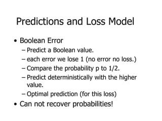
26. Predictions and Loss Model quadratic loss Predict a “real number” q for outcome 1. Loss (q-p) 2 for outcome 1 Loss ([1-q]-[1-p]) 2 for outcome 0 Expected loss: (p-q) 2 Minimized for p=q (Optimal prediction) recovers the probabilities Needs to know p to compute loss!

27. Predictions and Loss Model Logarithmic loss Predict a “real number” q for outcome 1. Loss log 1/q for outcome 1 Loss log 1/(1-q) for outcome 0 Expected loss: -p log q -(1-p) log (1-q) Minimized for p=q (Optimal prediction) recovers the probabilities Loss does not depend on p!

28. The basic PAC Model Unknown target function f(x) Distribution D over domain X Goal: find h(x) such that h(x) approx. f(x) Given H find h  H that minimizes Pr D [h(x)  f(x)]

29. Basic PAC Notions S - sample of m examples drawn i.i.d using D True error  (h)= Pr D [h(x)=f(x)] Observed error  ’(h)= 1/m |{ x  S | h(x)  f(x) }| Example (x,f(x)) Basic question: How close is  (h) to  ’(h)

30. Bayesian Theory Prior distribution over H Given a sample S compute a posterior distribution: Maximum Likelihood (ML) Pr[S|h] Maximum A Posteriori (MAP) Pr[h|S] Bayesian Predictor  h(x) Pr[h|S] .

31. Nearest Neighbor Methods Classify using near examples. Assume a “structured space” and a “metric” + + + + - - - - ?

32. Computational Methods How to find an h e H with low observed error. Heuristic algorithm for specific classes. Most cases computational tasks are provably hard.

33. Separating Hyperplane Perceptron: sign(  x i w i ) Find w 1 .... w n Limited representation x 1 x n w 1 w n  sign

34. Neural Networks Sigmoidal gates : a=  x i w i and output = 1/(1+ e -a ) Back Propagation x 1 x n

35. Decision Trees x 1 > 5 x 6 > 2 +1 -1 +1

36. Decision Trees Limited Representation Efficient Algorithms. Aim: Find a small decision tree with low observed error.

37. Decision Trees PHASE I: Construct the tree greedy, using a local index function. Ginni Index : G(x) = x(1-x), Entropy H(x) ... PHASE II: Prune the decision Tree while maintaining low observed error. Good experimental results

38. Complexity versus Generalization hypothesis complexity versus observed error. More complex hypothesis have lower observed error, but might have higher true error.

39. Basic criteria for Model Selection Minimum Description Length  ’ (h) + |code length of h| Structural Risk Minimization:  ’ (h) + sqrt{ log |H| / m }

40. Genetic Programming A search Method. Local mutation operations Cross-over operations Keeps the “best” candidates. Change a node in a tree Replace a subtree by another tree Keep trees with low observed error Example: decision trees

41. General PAC Methodology Minimize the observed error. Search for a small size classifier Hand-tailored search method for specific classes.

42. Weak Learning Small class of predicates H Weak Learning: Assume that for any distribution D , there is some predicate h  H that predicts better than 1/2+  . Weak Learning Strong Learning

43. Boosting Algorithms Functions: Weighted majority of the predicates. Methodology: Change the distribution to target “hard” examples. Weight of an example is exponential in the number of incorrect classifications. Extremely good experimental results and efficient algorithms.

44. Support Vector Machine n dimensions m dimensions

45. Support Vector Machine Use a hyperplane in the LARGE space. Choose a hyperplane with a large MARGIN. + + + + - - - Project data to a high dimensional space.

46. Other Models Membership Queries x f(x)

47. Fourier Transform f(x) =  z  z (x)  z (x) = (-1) <x,z> Many Simple classes are well approximated using large coefficients. Efficient algorithms for finding large coefficients.

48. Reinforcement Learning Control Problems. Changing the parameters changes the behavior. Search for optimal policies.

49. Clustering: Unsupervised learning

50. Unsupervised learning: Clustering

51. Basic Concepts in Probability For a single hypothesis h: Given an observed error Bound the true error Markov Inequality Chebyshev Inequality Chernoff Inequality

52. Basic Concepts in Probability Switching from h 1 to h 2 : Given the observed errors Predict if h 2 is better. Total error rate Cases where h 1 (x)  h 2 (x) More refine

53. Course structure Store observations in memory and retrieve Simple, little generalization (Distance measure?) Learn a set of rules and apply to new data Sometimes difficult to find a good model Good generalization Estimate a “flexible model” from the data Generalization issues, data size issues