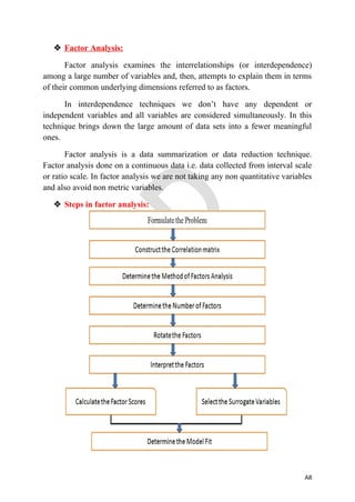
Factor analysis is a technique used to summarize a large set of variables by identifying underlying factors that explain their interrelationships. It involves constructing a correlation matrix between variables and using statistical methods like principal component analysis or common factor analysis to determine the number of factors needed to account for the variance within the data. The factors are then rotated and interpreted based on which original variables have the highest loadings on each factor. Factor analysis can reduce variables, validate scales, and select subsets of important variables.

1.  Factor Analysis:
Factor analysis examines the interrelationships (or interdependence)
among a large number of variables and, then, attempts to explain them in terms
of their common underlying dimensions referred to as factors.
In interdependence techniques we don’t have any dependent or
independent variables and all variables are considered simultaneously. In this
technique brings down the large amount of data sets into a fewer meaningful
ones.
Factor analysis is a data summarization or data reduction technique.
Factor analysis done on a continuous data i.e. data collected from interval scale
or ratio scale. In factor analysis we are not taking any non quantitative variables
and also avoid non metric variables.
 Steps in factor analysis:
AR

2. 1) Formulate the problem:
Identify the purpose of factor analysis. On the basis of fast research,
theory and judgement of the researcher specify the variables which are included
in the factor analysis. The selected variables must be properly measured on an
interval or ratio scale. The suitable sample size must be used. The sample size
should be at least four or five times in respect to the available variables.
2) Construct the correlation matrix:
A matrix of correlation between the variables is the basis of the analytical
process. The variables must be correlated for the suitable factor analysis. The
factor analysis would not be suitable if the correlation among all the variables is
small.
3) Determine the method of factor analysis:
i) Principal components analysis: In this approach the total variance
(unique variance and error variance and shared/common variance) in the data is
considered. When the analysis of data focuses to find the minimum number of
factors then principal component analysis is used. These factors will account for
maximum variance in the data for use in subsequent multivariate analysis.
ii) Common factor analysis: In this approach the common variance is
the basis of estimated factors. When the purpose of analysis is to identify the
underlying dimensions and the common variance then this approach is used.
This method is also known as principal axis factoring.
4) Determine the number of factors:
i) A priori determination: Sometimes on the basis of prior knowledge
the researcher knows that how many factors are required and hence a number of
factors are removed by the researcher to find the required number of factors.
ii) Determination based on Eigen values: In this approach, only those
factors are included whose Eigen values are greater than 1.0 and other factors
are not included in the model. The amount of variance which is associated with
the factor is called Eigen value.
iii) Determination based on Scree plot: The plotting of the Eigen values
against the number of factors for removing the unnecessary factors is called
scree plot. The number of factors is determined with the help of the shape of the
AR

3. plot. Typically, the plot has a distinct break between the steep slope of factors,
with large Eigen values and a gradual trailing-off associated with the rest of the
factors.
iv) Determination based on percentage of variance: In this approach,
determine the level of factors which is to be removed so that the cumulative
percentage of variance extracted by the factors reaches a satisfactory level. It is
suggested that the factors extracted should account for at least 60% of the
variance .
5) Rotate the factors :
The relationship between the factors and individual variables are
represented by the initial or unrotated factor matrix.
Different methods of rotation may result in the identification of different
factors. They are
i) Orthogonal rotation: If the axes are at right angle to each other then
rotation will be orthogonal.
ii) Oblique rotation: If the axes are not at right angle to each other than
the rotation will be diagonal and the factors will be correlated. When factors in
population are likely to be strongly correlated then the diagonal rotation should
be used.
6) Interpret factors:
Interpretation is facilitated with identification of the variables that have
large loadings on the same factor.
7) Calculate factor scores:
A linear combination of original variables is simply known as a factor.
The factor scores for the ith
factor may be estimated as follows
Fi=Wi1X1+Wi2X2+Wi3X3+...+WikXk
8) Select surrogate variables:
Sometimes, the researcher wants to select the surrogate variables instead
of computing factor scores. Selection of surrogate variables involves singling-
out some of the original variables for use in subsequent analysis.This allows the
AR

4. researcher to conduct subsequent analysis and results are interpreted in terms of
original variables rather than factor scores.
9) Determine the model fit:
To determine model fit examines the differences between the observed
correlations (as given in the input correlation matrix) and the reproduced
correlations (as estimated from the factor matrix).These differences are called
residuals. If there are many large residuals, the factor model does not provide a
good fit to the data and the model should be reconsidered.
 Applications of factor analysis:
1) To reduce a large number of variables to a small number of factors for data
modelling
2) To validate a scale by demonstrating that its constituent items load on the
same factor and to drop proposed scale items which cross load on more than one
factor.
3) To select a subset of variables from a larger set based on which original
variables have the highest correlations with the principal component factors.
AR