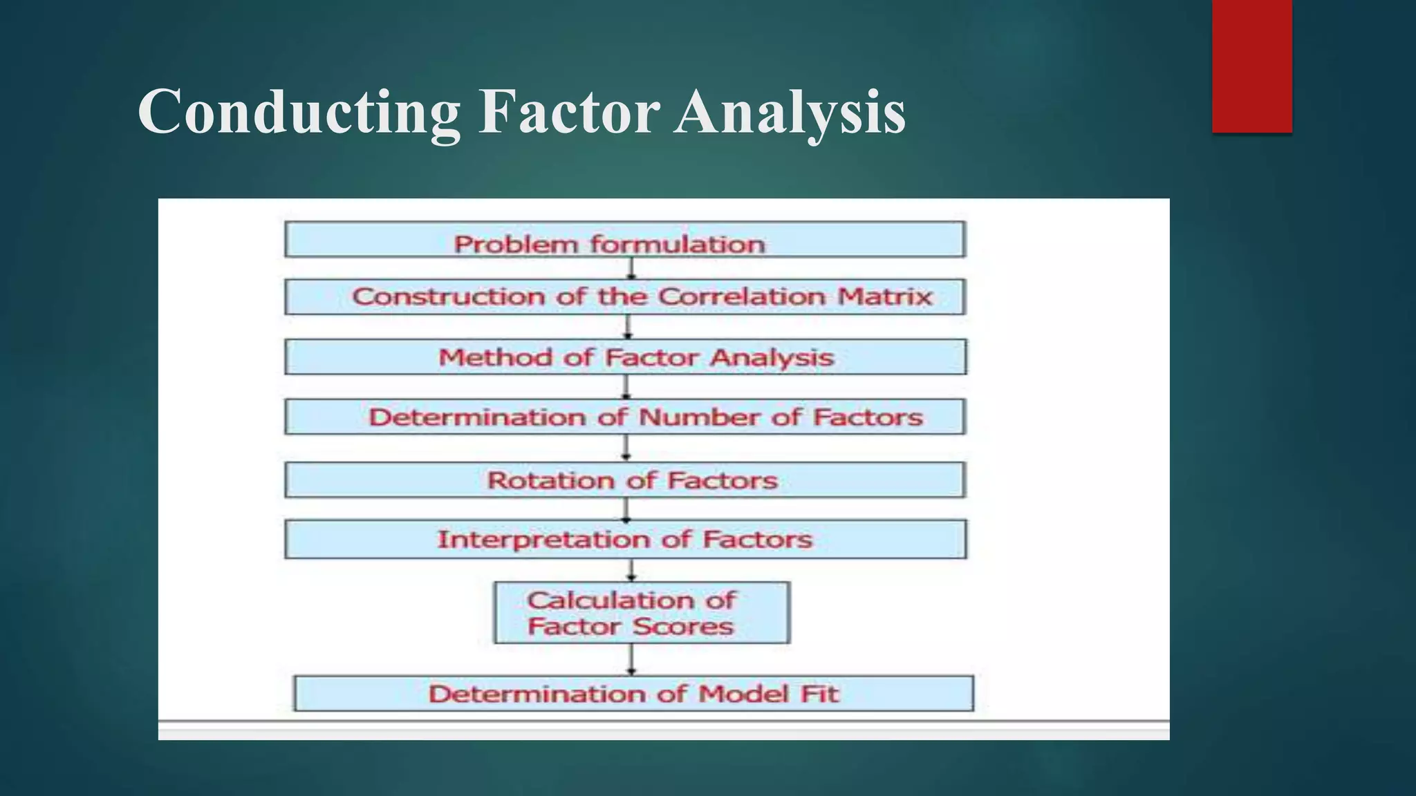
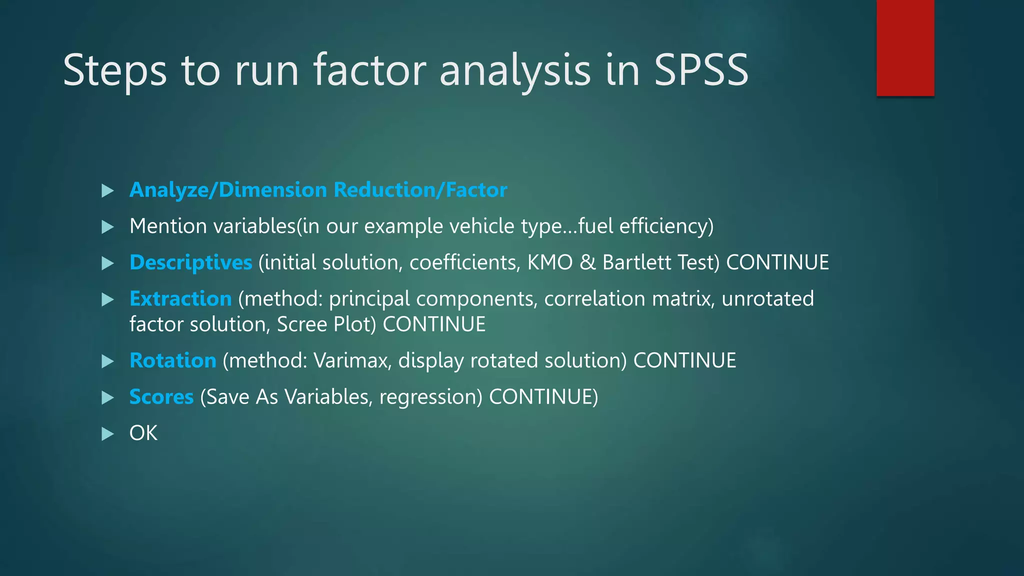
Factor analysis is a technique that is used to reduce a large number of variables into fewer numbers of factors. The basic assumption of factor analysis is that for a collection of observed variables there are a set of underlying variables called factors (smaller than the observed variables), that can explain the interrelationships among those variables.
Factor Extraction method in factor analysis with example in R studio.pptxGauravRajole
In this ppt information about factor analysis is given which is part of multivariate analysis. detail description is given about the factor extraction method, a test of the sufficiency of factor numbers, Interpretation of factors, factor score, rotation of factors, orthogonal rotation methods, varimax rotation, Oblique Rotation, and an example of factor analysis in R-studio.
Your Paper was well written, however; I need you to follow the frochellscroop
Your Paper was well written, however; I need you to follow the following Analysis Guidance for Intervention Data. I will give you a passing grade when you submit with these by the 26th of April at 1pm EST
This document is designed to provide a summary of the key steps for analysing intervention data. The main analysis is conducted using the general linear model function in SPSS. This document does not cover how to clean data for analysis. (Data for the PARS module has already been cleaned so students do not have to undertake this part of the analysis.) This document is written with the PARS assignment in mind, so please refer to statistical texts for details on how to check assumptions, and a broader overview of how to interpret the output of intervention analyses in SPSS.
Preparing Scales
When using scales, ensure you compute scale reliabilities (Cronbachs Alpha using the function Analyse>Scale>Reliability analysis). Make sure scales are recoded as required by the specific scale you’re using. If you find poor reliability, that might indicate scale items have not been coded as required (e.g. a scale item may need reverse coding). If scale reliability is poor, then you may want to exclude it from the analysis, remove a low-loading item, or report why you think the reliability is poor and justify why you decided to include it. Scale items should be aggregated or averaged using the compute variable function in SPSS (Transform>Compute variable) for the main analysis, as directed by the scale authors. (For the PARS assignment, scale reliability statistics can be reported in the appendix.)
Calculating Means and Standard Deviations
It is useful at this stage to calculate the means and standard deviations for the data using the function Analyse>Descriptive Statistics. For intervention data comparing more than one condition, you need to isolate a condition in the dataset before generating the means and standard deviations for that condition. The analyses testing the effect of an intervention with individuals in different conditions (i.e. between-subject) are essentially testing whether there is a significant difference in the means of groups in different conditions. The means for the different conditions show whether levels are increasing or decreasing, and this is useful for interpreting the results of the analysis.
Isolate study conditions using the function Data>Select cases, and use the function ‘If condition satisfied’. In the PARS data, use cohort as the variable in the rule (i.e. ‘Cohort = 1’ for the intervention group, or ‘Cohort = 2’ for the control group). When you have either of these rules applied, SPSS will only run the analysis on the cases selected by that rule. For example, if the rule applied is ‘Cohort = 1’ only cases with the value 1 in the cohort variable will be included in the analysis.
Bivariate Correlations
As part the analysis, you need to run bivariate correlations. Use the function Analyse>Correlate>Bivariate. (For ...
Multiple Linear Regression: a powerful statistical tool to understand and imp...Monica Mazzoni
It is known that, over time, all production processes tend to deviate from their initial conditions. This happens for the most diverse reasons:
changes in materials, personnel, environment,
technological improvements,
acquisition of production experience, etc.
Among other things, it is precisely in these changes that the foundations for an improvement of the process itself lie.
Week 5 Lecture 14 The Chi Square TestQuite often, patterns of .docxcockekeshia
Week 5 Lecture 14
The Chi Square Test
Quite often, patterns of responses or measures give us a lot of information. Patterns are generally the result of counting how many things fit into a particular category. Whenever we make a histogram, bar, or pie chart we are looking at the pattern of the data. Frequently, changes in these visual patterns will be our first clues that things have changed, and the first clue that we need to initiate a research study (Lind, Marchel, & Wathen, 2008).
One of the most useful test in examining patterns and relationships in data involving counts (how many fit into this category, how many into that, etc.) is the chi-square. It is extremely easy to calculate and has many more uses than we will cover. Examining patterns involves two uses of the Chi-square - the goodness of fit and the contingency table. Both of these uses have a common trait: they involve counts per group. In fact, the chi-square is the only statistic we will look at that we use when we have counts per multiple groups (Tanner & Youssef-Morgan, 2013). Chi Square Goodness of Fit Test
The goodness of fit test checks to see if the data distribution (counts per group) matches some pattern we are interested in. Example: Are the employees in our example company distributed equal across the grades? Or, a more reasonable expectation for a company might be are the employees distributed in a pyramid fashion – most on the bottom and few at the top?
The Chi Square test compares the actual versus a proposed distribution of counts by generating a measure for each cell or count: (actual – expected)2/actual. Summing these for all of the cells or groups provides us with the Chi Square Statistic. As with our other tests, we determine the p-value of getting a result as large or larger to determine if we reject or not reject our null hypothesis. An example will show the approach using Excel.
Regardless of the Chi Square test, the chi square related functions are found in the fx Statistics window rather than the Data Analysis where we found the t and ANOVA test functions. The most important for us are:
· CHISQ.TEST (actual range, expected range) – returns the p-value for the test
· CHISQ.INV.RT(p-value, df) – returns the actual Chi Square value for the p-value or probability value used.
· CHISQ.DIST.RT(X, df) – returns the p-value for a given value.
When we have a table of actual and expected results, using the =CHISQ.TEST(actual range, expected range) will provide us with the p-value of the calculated chi square value (but does not give us the actual calculated chi square value for the test). We can compare this value against our alpha criteria (generally 0.05) to make our decision about rejecting or not rejecting the null hypothesis.
If, after finding the p-value for our chi square test, we want to determine the calculated value of the chi square statistic, we can use the =CHISQ.INV.RT(probability, df) function, the value for probability is .
An overview of the significance of SURE(Seemingly unrelated regression) model in Panel data econometrics and its applications.
The presentation consists of the theoretical background and mathematical derivation for the model. The stochastic frontier model and treatment effects are also discussed in brief.
ViewShift: Hassle-free Dynamic Policy Enforcement for Every Data LakeWalaa Eldin Moustafa
Dynamic policy enforcement is becoming an increasingly important topic in today’s world where data privacy and compliance is a top priority for companies, individuals, and regulators alike. In these slides, we discuss how LinkedIn implements a powerful dynamic policy enforcement engine, called ViewShift, and integrates it within its data lake. We show the query engine architecture and how catalog implementations can automatically route table resolutions to compliance-enforcing SQL views. Such views have a set of very interesting properties: (1) They are auto-generated from declarative data annotations. (2) They respect user-level consent and preferences (3) They are context-aware, encoding a different set of transformations for different use cases (4) They are portable; while the SQL logic is only implemented in one SQL dialect, it is accessible in all engines.
#SQL #Views #Privacy #Compliance #DataLake
Unleashing the Power of Data_ Choosing a Trusted Analytics Platform.pdfEnterprise Wired
In this guide, we'll explore the key considerations and features to look for when choosing a Trusted analytics platform that meets your organization's needs and delivers actionable intelligence you can trust.
06-04-2024 - NYC Tech Week - Discussion on Vector Databases, Unstructured Data and AI
Discussion on Vector Databases, Unstructured Data and AI
https://www.meetup.com/unstructured-data-meetup-new-york/
This meetup is for people working in unstructured data. Speakers will come present about related topics such as vector databases, LLMs, and managing data at scale. The intended audience of this group includes roles like machine learning engineers, data scientists, data engineers, software engineers, and PMs.This meetup was formerly Milvus Meetup, and is sponsored by Zilliz maintainers of Milvus.
The Building Blocks of QuestDB, a Time Series Databasejavier ramirez
Talk Delivered at Valencia Codes Meetup 2024-06.
Traditionally, databases have treated timestamps just as another data type. However, when performing real-time analytics, timestamps should be first class citizens and we need rich time semantics to get the most out of our data. We also need to deal with ever growing datasets while keeping performant, which is as fun as it sounds.
It is no wonder time-series databases are now more popular than ever before. Join me in this session to learn about the internal architecture and building blocks of QuestDB, an open source time-series database designed for speed. We will also review a history of some of the changes we have gone over the past two years to deal with late and unordered data, non-blocking writes, read-replicas, or faster batch ingestion.
Global Situational Awareness of A.I. and where its headedvikram sood
You can see the future first in San Francisco.
Over the past year, the talk of the town has shifted from $10 billion compute clusters to $100 billion clusters to trillion-dollar clusters. Every six months another zero is added to the boardroom plans. Behind the scenes, there’s a fierce scramble to secure every power contract still available for the rest of the decade, every voltage transformer that can possibly be procured. American big business is gearing up to pour trillions of dollars into a long-unseen mobilization of American industrial might. By the end of the decade, American electricity production will have grown tens of percent; from the shale fields of Pennsylvania to the solar farms of Nevada, hundreds of millions of GPUs will hum.
The AGI race has begun. We are building machines that can think and reason. By 2025/26, these machines will outpace college graduates. By the end of the decade, they will be smarter than you or I; we will have superintelligence, in the true sense of the word. Along the way, national security forces not seen in half a century will be un-leashed, and before long, The Project will be on. If we’re lucky, we’ll be in an all-out race with the CCP; if we’re unlucky, an all-out war.
Everyone is now talking about AI, but few have the faintest glimmer of what is about to hit them. Nvidia analysts still think 2024 might be close to the peak. Mainstream pundits are stuck on the wilful blindness of “it’s just predicting the next word”. They see only hype and business-as-usual; at most they entertain another internet-scale technological change.
Before long, the world will wake up. But right now, there are perhaps a few hundred people, most of them in San Francisco and the AI labs, that have situational awareness. Through whatever peculiar forces of fate, I have found myself amongst them. A few years ago, these people were derided as crazy—but they trusted the trendlines, which allowed them to correctly predict the AI advances of the past few years. Whether these people are also right about the next few years remains to be seen. But these are very smart people—the smartest people I have ever met—and they are the ones building this technology. Perhaps they will be an odd footnote in history, or perhaps they will go down in history like Szilard and Oppenheimer and Teller. If they are seeing the future even close to correctly, we are in for a wild ride.
Let me tell you what we see.
06-04-2024 - NYC Tech Week - Discussion on Vector Databases, Unstructured Data and AI
Round table discussion of vector databases, unstructured data, ai, big data, real-time, robots and Milvus.
A lively discussion with NJ Gen AI Meetup Lead, Prasad and Procure.FYI's Co-Found
Enhanced Enterprise Intelligence with your personal AI Data Copilot.pdfGetInData
Recently we have observed the rise of open-source Large Language Models (LLMs) that are community-driven or developed by the AI market leaders, such as Meta (Llama3), Databricks (DBRX) and Snowflake (Arctic). On the other hand, there is a growth in interest in specialized, carefully fine-tuned yet relatively small models that can efficiently assist programmers in day-to-day tasks. Finally, Retrieval-Augmented Generation (RAG) architectures have gained a lot of traction as the preferred approach for LLMs context and prompt augmentation for building conversational SQL data copilots, code copilots and chatbots.
In this presentation, we will show how we built upon these three concepts a robust Data Copilot that can help to democratize access to company data assets and boost performance of everyone working with data platforms.
Why do we need yet another (open-source ) Copilot?
How can we build one?
Architecture and evaluation
Analysis insight about a Flyball dog competition team's performanceroli9797
Insight of my analysis about a Flyball dog competition team's last year performance. Find more: https://github.com/rolandnagy-ds/flyball_race_analysis/tree/main
2. Factor analysis
Factor analysis is a class of procedures used for data reduction and
summarization.
It is an interdependence technique: no distinction between
dependent and independent variables.
Factor analysis is used:
To identify underlying dimensions, or factors, that explain the correlations among a set
of variables.
To identify a new, smaller, set of uncorrelated variables to replace the original set of
correlated variables.
3. Types of factor analysis
Exploratory Factor Analysis :- Researchers are not aware of how many
underlying dimensions( Factors) can be found from the variables that are under
study. Depending upon the co linearity between the variables limited number of
factors are derived.
Confirmatory Factor Analysis :- In this analysis researchers test the hypothesis
whether the variables under study based on theoretical support actually conform
to the factor structure or not.
4. Methods used for factor analysis in
SPSS
In Principal components analysis(mostly preferred) the total variance in the data is
considered.
-Used to determine the min number of factors that will account for max variance in the
data.
It is the most common method which the researchers use. Also, it extracts the maximum
variance and put them into the first factor. Subsequently, it removes the variance explained
by the first factor and extracts the second factor. Moreover, it goes on until the last factor.In
Common factor analysis, the factors are estimated based only on the common variance.
6. Factor Analysis Model
Each variable is expressed as a linear combination of factors. The factors are some
common factors plus a unique factor. The factor model is represented as:
Xi = Ai 1F1 + Ai 2F2 + Ai 3F3 + . . . + AimFm + ViUi
where
Xi = i th standardized variable
Aij = standardized mult reg coeff of var i on common factor j
Fj = common factor j
Vi = standardized reg coeff of var i on unique factor i
Ui = the unique factor for variable i
m = number of common factors
7. Statistics in factor analysis
Bartlett's test of sphericity. Bartlett's test of sphericity is used to test the
hypothesis that the variables are uncorrelated in the population (i.e., the population
corr matrix is an identity matrix)
Correlation matrix. A correlation matrix is a lower triangle matrix showing the
simple correlations, r, between all possible pairs of variables included in the
analysis. The diagonal elements are all 1.
8. Communality. Amount of variance a variable shares with all the other variables.
This is the proportion of variance explained by the common factors.
Eigenvalue. Represents the total variance explained by each factor.
Factor loadings. Correlations between the variables and the factors.
Factor matrix. A factor matrix contains the factor loadings of all the variables on
all the factors
9. Factor scores. Factor scores are composite scores estimated for each respondent
on the derived factors.
Kaiser-Meyer-Olkin (KMO) measure of sampling adequacy. Used to examine
the appropriateness of factor analysis. High values (between 0.5 and 1.0) indicate
appropriateness. Values below 0.5 imply not.
Percentage of variance. The percentage of the total variance attributed to each
factor.
Scree plot. A scree plot is a plot of the Eigenvalues against the number of factors
in order of extraction.
10. Steps to run factor analysis in SPSS
Analyze/Dimension Reduction/Factor
Mention variables(in our example vehicle type…fuel efficiency)
Descriptives (initial solution, coefficients, KMO & Bartlett Test) CONTINUE
Extraction (method: principal components, correlation matrix, unrotated
factor solution, Scree Plot) CONTINUE
Rotation (method: Varimax, display rotated solution) CONTINUE
Scores (Save As Variables, regression) CONTINUE)
OK
11. Interpretations of factor analysis in
SPSS
• The next output from the analysis is the correlation coefficient. A correlation matrix is simply a
rectangular array of numbers that gives the correlation coefficients between a single variable and
every other variable in the investigation.
• The correlation coefficient between a variable and itself is always 1, hence the principal diagonal of
the correlation matrix contains 1s. The correlation coefficients above and below the principal
diagonal are the same.
12. KMO and Barlett’s Test
Kaiser-Meyer-Olkin Measure of Sampling Adequacy – It is an index used to examine
appropriateness of factor analysis.This measure varies between 0 and 1, and values closer to 1
are better.
Values equal to or greater than 0.5 indicate that factor analysis is appropriate.
Bartlett’s Test of Sphericity – This tests the null hypothesis that the correlation matrix is an
identity matrix. An identity matrix is matrix in which all of the diagonal elements are 1 and all
off diagonal elements are 0 that is the variables are uncorrelated in the population
You want to reject this null hypothesis.
the significance value should be is less than 0.05 to reject null hypothesis and conclude
that the variables are correlated in the population
13. Communalities
Communality is the amount of variance a variable shares with all the other variables being
considered. Small values indicate variables that do not fit well with the factor solution,
Extraction – The values in this column indicate the proportion of each variable’s variance that can be
explained by the retained factors. Variables with high values are well represented in the common factor
space, while variables with low values are not well represented. Here we can see that all extraction values
are high.
14. Total variance explained
The next item shows all the factors extractable from the analysis along with their eigenvalues,
the percent of variance attributable to each factor, and the cumulative variance of the factor
and the previous factors. Here we can three factors are selected because three factors have
eigen values greater than one 5.994,1.654 and 1.123
Eigen Value: The eigenvalue represents the total variance explained by each factor.
Factors having eigenvalues over 1 are selected for further study.
15. Scree plot
The scree plot is a graph of the eigenvalues against all the factors. The graph is useful for
determining how many factors to retain.
One rule is to consider only those points with eigenvalues over 1.
16. Component matrix
The elements of the Component Matrix are correlations of the item with each component.
• Summing the squared component loadings(correlations) across the components (columns)
gives you the communality estimates for each item,
• and summing each squared loading down the items (rows) gives you the eigenvalue for each
component.
17. Rotations
ORTHOGONAL ROTATION- Rotations that assume the factors are not
correlated are called orthogonal rotations(Axes maintained at right
angles(varimax is a popular choice)
OBLIQUE ROTATION- Rotations that allow for correlation between
factors are called oblique rotations(. Axes not maintained at right angles)
18. Rotated component matrix
The idea of rotation is to reduce the number factors on which the variables under
investigation have high loadings.
The maximum of each row(excluding the sign) shows that the particular variable belongs
to the respective component
Example: vehicle type has the maximum value 0.954 under factor 3 so it belongs to factor
three
19. Try it yourself:
Example-2(Toothpaste data file)
To determine benefits from toothpaste
Responses were obtained on 6 variables:
V1: It is imp to buy toothpaste to prevent cavities
V2: I like a toothpaste that gives shiny teeth
V3: A toothpaste should strengthen your gums
V4: I prefer a toothpaste that freshens breath
V5: Prevention of tooth decay is not imp
V6: The most imp consideration is attractive teeth
Responses on a 7-pt scale (1=strongly disagree; 7=strongly agree)