Excel tips

Getting started With ExcelGetting started With Excel

Know your Worksheet
Formatting Cells In Excel
Go To Cells Quickly
Select Cells
Enter Data
Edit a Cell
Wrap Text
Delete a Cell
Entry
Save a File
Close Excel

Working with Excel worksheet
Hide / Unhide a sheet
Rename a sheet

Add color to sheet tabs Conditional formatting
Move or copy sheets

Uncheck to hide
gridlines
Show or hide gridlines on a worksheet
Change the color of
gridlines

Formatting Cells in Excel
When you enter data into a cell in Excel, it is handled differently depending on what type of formatting you
have assigned to the cell. For example, if you choose Currency formatting, Excel will automatically convert
3 into $3.00; if you choose Date formatting, Excel would convert 3/1 to March 1, 2009; and if you
choose Percent formatting, Excel would change 0.3 to 30%.
All of these choices are available when you highlight/select the cell(s) you want to format, then go to
the Format menu and choose Cells, then click on the Number tab in the Format Cells dialog box. There is
also a choice named Special and when you choose that, you can select formats like Social Security Number,
Phone Number, etc.
But, what if you want a format that is not included in Excel's pre-made formats? Well, you can make your
own custom format, following the directions below.
Type the number 123456789 in an empty
cell and hit Enter. Now click back onto
that cell and go to the Format Menu and
select Cells. Click on the Number tab and
select Custom from the list.
In the box on the left, see all the
different custom formats Excel offers.
There are formats in here for most of
the styles you would get if you chose one
of the options for any of the choices in
the list on the left. For example, in the
list on the right, there is a custom format
that is simply an @ symbol. If you choose
this, it simply formats your cell as text. I
recommend you look through the list and
try some of them and see how they
affect the number 123456789 that you
have typed in your cell. Since there are so
many, I can't possibly go through all of
them with you. But, what I do want to do
is teach you how to make some of your
own.

Go To Cells Quickly
The following are shortcuts for moving quickly from one cell in a worksheet to a cell in a different
part of the worksheet.
EXERCISE 2
Go to -- F5
The F5 function key is the "Go To" key. If you press the F5 key, you are prompted for the cell to
which you wish to go. Enter the cell address, and the cursor jumps to that cell.
Press F5. The Go To dialog box opens.
Type J3 in the Reference field.
Press Enter. Excel moves to cell J3.
Go to -- Ctrl+G
You can also use Ctrl+G to go to a specific cell.
Hold down the Ctrl key while you press "g" (Ctrl+g). The Go To dialog box opens.
Type C4 in the Reference field.
Press Enter. Excel moves to cell C4.
The Name Box
You can also use the Name box to go to a specific cell. Just type the cell you want to go to in the
Name box and then press Enter.
Type B10 in the Name box.
Press Enter. Excel moves to cell B10.

Select Cells
If you wish to perform a function on a group
of cells, you must first select those cells by
highlighting them. The exercises that follow
teach you how to select.
EXERCISE 3
Select Cells
To select cells A1 to E1:
1.Go to cell A1.
2.Press the F8 key. This anchors the cursor.
3.Note that "Extend Selection" appears on the
Status bar in the lower-left corner of the window.
You are in the Extend mode.
4.Click in cell E7. Excel highlights cells A1 to E7.
5.Press Esc and click anywhere on the
worksheet to clear the highlighting.
Alternative Method: Select Cells by Dragging
You can also select an area by holding down the
left mouse button and dragging the mouse over
the area. In addition, you can select
noncontiguous areas of the worksheet by doing
the following:
Go to cell A1.
Hold down the Ctrl key. You won't release it until step 9.
Holding down the Ctrl key enables you to select
noncontiguous areas of the worksheet.
Press the left mouse button.
While holding down the left mouse button, use the mouse
to move from cell A1 to C5.
Continue to hold down the Ctrl key, but release the left
mouse button.
Using the mouse, place the cursor in cell D7.
Press the left mouse button.
While holding down the left mouse button, move to cell
F10.
 Release the left mouse button.
Release the Ctrl key. Cells A1 to C5 and cells D7 to F10
are selected.
Press Esc and click anywhere on the worksheet to remove
the highlighting.

Enter Data
In this section, you will learn how to enter data into your worksheet. First, place the cursor in the cell in
which you want to start entering data. Type some data, and then press Enter. If you need to delete,
press the Backspace key to delete one character at a time.
EXERCISE 4
Enter Data
1.Place the cursor in cell A1.
2.Type John Jordan. Do not press Enter at this time.
Delete Data
The Backspace key erases one character at a time.
1.Press the Backspace key until Jordan is erased.
2.Press Enter. The name "John" appears in cell A1.

Edit a Cell
After you enter data into a cell, you can edit the data by pressing F2 while you are in the
cell you wish to edit.
EXERCISE 5
Edit a Cell
Change "John" to "Jones."
Move to cell A1.
Press F2.
Use the Backspace key to delete the "n" and the "h."
Type nes.
Press Enter.
Alternate Method: Editing a Cell by Using the Formula Bar
You can also edit the cell by using the Formula bar. You change "Jones" to "Joker" in the following
exercise.
1. Move the cursor to cell A1.
2. Click in the formula area of the Formula bar.
3. Use the backspace key to erase the "s," "e," and "n."
4. Type ker.
5. Press Enter.

Wrap Text
When you type text that is too long to fit in the cell, the text overlaps the next cell. If you do not want it
to overlap the next cell, you can wrap the text.
EXERCISE 6
Wrap Text

1.Move to cell A2.
2.Type Text too long to fit.
3.Press Enter.
1.Return to cell A2.
2.Choose the Home tab.
3.Click the Wrap Text button
4. Excel wraps the text in the cell.

Delete a Cell Entry
To delete an entry in a cell or a group of cells, you place the cursor in the cell or select the group of cells and press Delete.
EXERCISE 7
Delete a Cell Entry
Select cells A1 to A2.
Press the Delete key.
Save a File
This is the end of Lesson1.
To save your file:
Click the Office button. A menu appears.
Click Save. The Save As dialog box appears.
Go to the directory in which you want to save your file.
Type Lesson1 in the File Name field.
Click Save. Excel saves your file.
Close Excel
Close Microsoft Excel.
Click the Office button. A menu appears.
Click Close. Excel closes.

Calculating Data with Advanced FormulasCalculating Data with Advanced Formulas

NAMES
When entering formulae or referring to any area on the spreadsheet,
it is usual to refer to a "range".
For example, B6 is a range reference; B6:B10 is also a range reference.
Defining Names
There are a number of ways to set up names on a spreadsheet.
A common way is to use the Insert, Name, Define menu.
In the example, there is a range of sales figures that could be named “1st_Qtr”;
Selection of
cells for
naming

To name range:
i. Select the cells you wish to name.
ii. Click the DEFINE NAME button in the NAMES GROUP in the insert tab
iii. The DEFINE NAME dialog box appears
iv. To name the cells, simply type a name in the Name box and choose OK.
To manage names:
The Define Name Dialog box also lets you manage the range names you can add delete or modify the existing range
name in the same dialog box.

Go To
The GOTO feature can be used to go to a specific cell address on the spreadsheet. It can also be used in conjunction with
names.
i. Press [F5]. The following dialog box appears;
ii. Click on the name required, then choose OK.
Using Names
Not only does the cell pointer move to the correct range, but it
also selects it. This can be very useful for checking that ranges
have been defined correctly, and also for listing all the names on the
spreadsheet.

Names In Formulae
Names can be used in any simple formula, as well as any of Excel's built in functions.
Instead of typing cell references or selecting cells, simply type the name or paste the
name into the formula.

Excel Functions
CONDITIONAL & LOGICAL FUNCTIONS
If Statements
Logical Test
Value If True / False
Nested If
AND, OR, NOT
And
Or
Not
LOOKUP FUNCTIONS
Lookup
Hlookup
Vlookup
OTHER USEFUL FUNCTIONS
ISERROR TRIM
IFERROR NOW
COUNTIF RIGHT
AVERAGEIF LEFT
SUMIF Find & Replace
CONCATENATE

Absolute Cell Addressing
Before learning Excel formula we will study about absolute cell referencing in excel. In Excel, a reference to
a particular cell or group of cells that does not change, even if you change the shape or size of the
spreadsheet, or copy the reference to another cell. For example, the cell reference "$A$3" is an absolute
cell reference that always points to the cell in the first column and third row. In contrast, the reference
"A3" is a relative cell reference that initially points to the cell in the first column and third row, but may
change if you copy the reference to another cell .Absolute cell references are particularly useful for
referencing constant values (i.e., values that never change).
1.Move to cell C12.
2.Type =.
3.Click cell C9.
4.Press F4. Dollar signs appear before the C and the 9.
5.Type +.
6.Click cell C10.
8.Type +.
9.Click cell C11.
11.Click the check mark on the formula bar. Excel records the formula in cell C12.

CONDITIONAL & LOGICAL FUNCTIONS
Excel has a number of logical functions which allow you to set various "conditions" and have data
respond
to them. For example, you may only want a certain calculation performed or piece of text displayed if
certain conditions are met. The functions used to produce this type of analysis are found in the Insert,
Function menu, under the heading LOGICAL.

If Statements
The IF function is used to analyze data, test whether or not it meets certain conditions and then act upon
its decision.
the IF statement is accompanied by three arguments enclosed in one set of parentheses; the condition to be
met (logical_test); the action to be performed if that condition is true (value_if_true); the action to be
performed if false (value_if_false). Each of these is separated by a comma, as shown;
=IF ( logical_test, value_if_true, value_if_false)
Logical Test
This part of the IF statement is the "condition", or test. You may want to test to see if a cell is a certain
value, or to compare two cells. In these cases, symbols called LOGICAL OPERATORS are useful;
> Greater than
< Less than
> = Greater than or equal to
< = Less than or equal to
= Equal to
< > Not equal to

Nested If
When you need to have more than one condition and more than two possible outcomes, a NESTED IF is
required. This is based on the same principle as a normal IF statement, but involves "nesting" a secondary
formula inside the main one. The secondary IF forms the FALSE part of the main statement, as follows;
=IF(1st logic test , 1st true value , IF(2nd logic test , 2nd true value , false value))
Only if both logic tests are found to be false will the false value be returned. Notice that there are two
sets
of parentheses, as there are two separate IF statements. This process can be enlarged to include more
conditions and more eventualities up to seven IF's can be nested within the main statement. However,‐
care must be taken to ensure that the correct number of parentheses are added.
In the example, sales staff could now receive one of three possible ratings;
=IF(B2>1000,"GOOD",IF(B2<600,"POOR","AVERAGE"))
To make the above IF statement more flexible, the logical tests could be amended to measure sales
against
cell references instead of figures. In the example, column E has been used to hold the upper and lower
sales thresholds.
=IF(B2>$E$2,"GOOD",IF(B2<$E$3,"POOR","AVERAGE"))
(If the IF statement is to be copied later, this cell reference should be absolute).

Rather than create large and unwieldy formulae involving multiple IF statements, the AND, OR and NOT
functions can be used to group logical tests or "conditions" together. These three functions can be used on
their own, but in that case they will only return the values "TRUE" or "FALSE". As these two values are not
particularly meaningful on a spreadsheet, it is much more useful to combine the AND, OR and NOT functions
within an IF statement. This way, you can ask for calculations to be performed or other text messages to
appear as a result.
AND, OR, NOT

And
This function is a logical test to see if all conditions are true. If this is the case, the value "TRUE" is
returned. If any of the arguments in the AND statement are found to be false, the whole statement
produces the value "FALSE". This function is particularly useful as a check to make sure that all
conditions you set are met. Arguments are entered in the AND statement in parentheses, separated by
commas, and there is a maximum of 30 arguments to one AND statement. The following example checks
that two cells, B1 and B2, are both greater than 100.
=AND(B1>100,B2>100)
If either one of these two cells contains a value less than a hundred, the result of the AND statement is
"FALSE.” This can now be wrapped inside an IF function to produce a more meaningful result. You may
want to add the two figures together if they are over 100, or display a message indicating that they are
not high enough.
=IF(AND(B1>100,B2>100),B1+B2,"Figures not high enough")

Or
This function is a logical test to see if one or more conditions are true. If this is the case, the value
"TRUE" is returned. If just one of the arguments in the OR statement is found to be true, the whole
statement produces the value "TRUE". Only when all arguments are false will the value "FALSE" be
returned. This function is particularly useful as a check to make sure that at least one of the conditions
you set is met.
=IF(OR(B1>100,B2>100),"at least one is OK","Figures not high enough")
In the above formula, only one of the numbers in cells B1 and B2 has to be over 100 in order for them to be
added together. The message only appears if neither figure is high enough.

Not
NOT checks to see if the argument is false. If so, the value "TRUE" is returned. It is best to use NOT as
"provided this is not the case" function. In other words, so long as the argument is false, the overall
statement is true. In the example, the cell contents of B1 are returned unless the number 13 is
encountered. If B1 is found to contain 13, the message "Unlucky!" is displayed;
=IF(NOT(B1=13),B1,"Unlucky!")
The NOT function can only contain one argument. If it is necessary to check that more than one argument
is false, the OR function should be used and the true and false values of the IF statement reversed.
Suppose, for example, a check is done against the numbers 13 and 666;
=IF(OR(B1=13,B1=666),"Unlucky!",B1)

LOOKUP FUNCTIONS
These functions allow you to create formulae which examine large amounts of data and
find information which matches or approximates to certain conditions. They are simpler to
construct than nested IF’s and can produce many more varied results.

Lookup
The syntax for LOOKUP is as follows;
=LOOKUP( lookup_value , lookup_vector , result_vector )
number or text entry
to look for
area in which to
search for the
lookup_value
adjacent row or
column where the
corresponding
value or text is
to be found
It is essential that data in
the lookup vector is placed
in ascending order, i.e.
numbers from lowest
to highest, text from A to
Z. If this is not done, the
LOOKUP function may
return the wrong result.

In the diagram, column D contains varying salaries, against which there is a company car in column E which
corresponds to each salary. For example, a £20030 salary gets a Golf, a £35000 salary gets a Scorpio. A
LOOKUP formula can be used to return whatever car is appropriate to a salary figure that is entered. In this
case, the lookup_value is the cell where the salary is entered (B13), the lookup_vector is the salary column
(D3:D11), and the result_vector is the car column (E3:E11). Hence the formula;
=LOOKUP(B13,D3:D11,E3:E11)
Typing 40000 in cell B13 will set the lookup_value. LOOKUP will search through the lookup_vector to find
the matching salary, and return the appropriate car from the result_vector, which in this case is Mercedes.
Alternatively, the formula could be simplified and cell references avoided by using Formula, Define Name to
give appropriate range names. Call B13 Salary, D3:D11 Salaries and E3:E11 Cars. The LOOKUP formula could
then be simplified to;
=LOOKUP(Salary,Salaries,Cars)
One of the advantages of the LOOKUP function is that if the exact lookup_value is not found, it will
approximate to the nearest figure below the requested value. For instance, if a user enters a Salary of
23000, there is no figure in the Salaries range which matches this. However, the nearest salary below 23000
is 20030, so the corresponding car is returned, which is a Golf. This technique is very useful when the
lookup_vector indicates grades or "bands.” In this case, anyone in the salary "band" between 20030 and
25000 gets a Golf. Only when their salary meets or exceeds 25000 do they get a Sierra.
There may be occasions where the lookup_value is below the lowest
value in the vector. In this case the #N/A message is displayed.

Hlookup
The horizontal LOOKUP function (HLOOKUP) can be used not just on a "vector" (single column or row of
data), but on an "array" (multiple rows and columns).
The syntax for HLOOKUP is;
=HLOOKUP( lookup_value , table_array , row_index_number)
number or
text entry to
look for
cell references (or
range name) of the
entire table of data;
row from
which the
result is
required
as HLOOKUP searches horizontally (i.e. across the array),
data in the first row must be in ascending order, i.e. numbers from lowest to highest, text from A to Z. As
with LOOKUP, if this rule is ignored, HLOOKUP will return the wrong value.

Whatever the amount a customer wants to borrow, he may pay up to five different rates of interest
depending on whether the loan is over 10, 15 or more years. The HLOOKUP function will find a specific
amount, then move down the array to find the appropriate interest rate for the required time period.
Designate cell A51 as the cell to hold the amount, i.e. the lookup_value; cells C43:H48 are the table_array;
the row_index_number will be 2 if a customer wants the loan over 10 years, 3 if he wants the loan over 15
years, and so on. Cell B51 holds this formula;
=HLOOKUP(A51,C43:H48,3)
The above formula looks along the top row of the array for the value in cell A51 (30000). It then moves
down to row 3 and returns the value 15.00%, which is the correct interest rate for a £30000 loan over 15
years. (Range names could be used here to simplify the formula).
As with the LOOKUP function, the advantage of HLOOOKUP is that it does not necessarily have to find the
exact lookup_value. If, for example, you wanted to find out what interest rate is applicable to a £28000
loan, the figure 28000 can be entered in the lookup_value cell (A51) and the rate 14.30% appears. As
before, Excel has looked for the value in the array closest to, but lower than, the lookup_value.

Vlookup
The VLOOKUP function works on the same principle as HLOOKUP, but instead of searching horizontally,
VLOOKUP searches vertically.
The syntax for the VLOOKUP function follows the same pattern as HLOOKUP, except that instead of
specifying a row index number, you would specify a column index number to instruct VLOOKUP to move
across to a specific column in the array where the required value is to be found.
=VLOOKUP( lookup_value , table_array , col_index_number )
In the case of VLOOKUP, data in the first column of the array should be in ascending order, as VLOOKUP
searches down this column for the lookup_value.
In the same spreadsheet as before, a VLOOKUP formula could be used to search for a specific time period,
then return the appropriate rate for a fixed amount. In the following example, a time period is entered in
cell A54 and in B54 the VLOOKUP formula is contained;
Cell B54 holds this formula;
=VLOOKUP(A54,C43:H48,5)

The cell A54 is the lookup_value (time period), the table_array is as before, and for this example rates
are
looked up for a loan of £40000, hence the column_index_number 5. By changing the value of cell A54, the
appropriate rate for that time period is returned. Where the specific lookup_value is not found,
VLOOKUP
works in the same way as HLOOKUP. In other words, the nearest value in the array that is less than the
lookup_value will be returned. So, a £40000 loan over 17 years would return an interest rate of 16.00%.

ISERROR
ISERROR is a very useful function that tells you if the formula you look at with it gives any error value.
Iserror (Value)
Value refers to any error value (#N/A, #VALUE!, #REF!, #DIV/0!, #NUM!, #NAME?, or #NULL!)
To use ISERROR function
In the example below the average functions in the column G is trying to divide empty cells and giving the
error message #DIV/0! The error function checking that cell gives the value true there is an error this
could
be nested in an IF function with an AVERAGE function so that the error message does not show in column
G

IFERROR
IFERROR(Value, value_if_error)
A common request in the area of functions is something to simplify error checking.
E.G. If a user wants to catch errors in a VLOOKUP and use their own error text opposed to Excel’s error,
they have to do something like this using the IF and ISERROR functions:
=IF(ISERROR(VLOOKUP("Dave", SalesTable, 3, FALSE)), " Value not found", VLOOKUP("Dave",
SalesTable, 3, FALSE))
As you can see, users need to repeat the VLOOKUP formula twice. This has a number of problems.
FIRST, it is hard to read and hard to maintain – if you want to change a formula, you have to do it twice.
SECOND, it can affect performance, because formulas are quite often run twice. The IFERROR function
solves these problems, enabling customers to easily trap and handle formula errors.
Here is an example of how a user could use it in the same situation:
=IFERROR(VLOOKUP(“Bob”, SalesTable, 3, false), “Value not found”)

COUNTIF
COUNTIF counts the number of cells in a range based on given criteria.
COUNTIF(range,criteria)
RANGE is one or more cells to count, including numbers or names, arrays, or references that contain
numbers. Blank and text values are ignored.
CRITERIA is the criteria in the form of a number, expression, cell reference, or text that defines
which cells
will be counted. For example, criteria can be expressed as 32, "32", ">32", "apples", or B4.

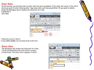
AVERAGEIF
A very common request is for a single function to conditionally average a range of numbers – a complement
to SUMIF and COUNTIF. AVERAGEIF, allows users to easily average a range based on a specific criteria.
AVERAGEIF(Range, Criteria, [Average Range])
RANGE is one or more cells to average, including numbers or names, arrays, or references that contain
numbers.
CRITERIA is the criteria in the form of a number, expression, cell reference, or text that defines which
cells are averaged. For example, criteria can be expressed as 32, "32", ">32", "apples", or B4.
AVERAGE range is the actual set of cells to average. If omitted, RANGE is used.
Here is an example that returns the average of B2:B5 where the corresponding value in column A is
greater
than 250,000:
=AVERAGEIF(A2:A5, “>250000”, B2:B5)

Sumif
the SumIf function adds all numbers in a range of cells, based on a given criteria.
The syntax for the SumIf function is:
SumIf( range, criteria, sum_range )
range is the range of cells that you want to apply the criteria against.
criteria is used to determine which cells to add.
sum_range are the cells to sum.
Based on the given example
=SumIf(A2:A6, D2, C2:C6)
would return 218.6
=SumIf(A:A, D2, C:C) would return 218.6
=SumIf(A2:A6, 2003, C2:C6) would return 7.2
=SumIf(A2:A6, ">=2001", C2:C6) would return 12.6

Concatenate
the Concatenate function allows you to join 2 or more strings together.
The syntax for the Concatenate function is:
Concatenate( text1, text2, ... text_n )
There can be up to 30 strings that are joined together.
=Concatenate(A1, A2)
would return "Alphabet"
=Concatenate (A2,”
“ ,”ter”)
would return “bet ter”
=Concatenate(A1, "bet
soup")
would return "Alphabet
soup"

Trim Function
the Trim function returns a text value with the leading and trailing spaces removed.
The syntax for the Trim function is:
=Trim( text )
text is the text value to remove the leading and trailing spaces from.
=Trim(A1)
would return "Tech on the Net"
=Trim(A2) would return "1234"
=Trim(A3) would return "alphabet soup"
=Trim(" apples ") would return "apples"
Now Function
the Now function returns the current system
date and time.
The syntax for the Now function is:
=Now()

Right Function
the Right function extracts a substring from a string starting from the
right-most character.
The syntax for the Right function is:
=Right( text, number_of_characters )
text is the string that you wish to extract from.
number_of_characters indicates the number of characters that you wish
to extract starting from the right-most character.
=Right(A1, 4)
would return "soup"
=Right(A2, 6) would return "thenet"
=Right ("Excel", 3) would return "cel"
Left Function

Data Presentation-Charting AbilityData Presentation-Charting Ability

Data Presentation
• Create embedded charts
• Create separate page charts
• Change chart types and formats
• Add and remove chart data
• Add trend lines to charts
• Create picture charts
One of the most impressive aspects of Excel is its charting ability. There are endless variations available,
allowing you to produce a chart, edit and format it, include notes, arrows, titles and various other extras as
desired.
We will learn to :-

Terminology
As a starting point, there are some terms used in charting which should be understood by you. The terms
defined below relate to the example car sales worksheet and column chart which appear beneath the table:
Data Point : An individual figure on the spreadsheet which is reflected in the chart e.g. Fred's Orion sales
figure
Data Series : A collection of related data points, e.g. all of Fred's figures, which will appear on a chart as
markers (bars, for example) of the same colour.
Legend: The "key" to the chart, identifying which patterns/colours relate to which data series Marker A bar,
column, or slice of pie for example, representing a data point.
Category: The category axis appears across the bottom of a graph (pie charts excepted) and the categories are
listed here. Points within the different data series are grouped by category

Embedded Charts
An embedded chart appears on the worksheet where it was created. It is an embedded object, which does
not normally appear in its own window, and has no separate existence apart from the worksheet.
All charts whether embedded or separate are created from the INSERT ribbon in the
CHARTS group.

Separate Chart Pages
A chart sheet, although linked to the worksheet whose figures it represents, exists as a separate page in a
workbook. The F11 key is very useful for creating a default chart from selected data as a new sheet within
the workbook
Some Chart Elements
area where you can
specify the titles to
have on the chart
Here you specify whether you
want a Y/Z axis and whether you
are using
timescales to plot your data
The gridline ribbon allows you to switch on and
off horizontal and vertical gridlines
Use this ribbon to switch the
legend on and off or reposition it
The Data Labels ribbon allows you to display the
amount each point represents or display the label
The Data Table ribbon will display a
grid underneath the chart that will
show the
information that is being plotted.

Methods To Create Charts
To create a chart
Mouse
i. Select data for chart.
ii. Go to the CHARTS group on the INSERT ribbon. Select
a chart type and click
iii. The menu on the left appears.
iv. Hovering your mouse over a chart type will bring up an
explanation of that chart type
v. When you have chosen click once to select a chart type
vi. The chart is now created based on the selected data as
an embedded chart.
OR
Keyboard
i. Select Data for chart
ii. Press the F11 Key
iii. Default chart will created as chart on a separate sheet.

Chart Types
There are several different types of chart available within Excel. The type to choose will vary depending
on
the data involved and what information the chart is intended to convey or highlight.
Area
Area charts can be 2 or 3dimensional. They are used to compare the change in volume of a
data series over time, emphasising the amount of change rather than the rate of change.
Bar
Bar charts can be 2 or 3Dimensional. They are used to show individual figures at a specific
time or to compare different items.
Column
Column charts can be 2 or 3 Dimensional. They are frequently used to show variation of‐
different items over a period of time.
Line
Line charts can be 2 or 3 Dimensional. Line charts are used to compare trends over time.‐
Pie
Pie charts can be 2 or 3Dimensional. They are used to compare the size of the parts with
the whole. Only one data series can be plotted, making up 100%.

Radar
Each category in a radar chart has its own axis radiating from the centre point. Data
points are plotted along each spoke, and data points belonging to the same series are
connected by lines.
Xy Scatter Charts
XY charts are used to compare two different numeric data series, and can be useful in
determining whether one set of figures might be dependent on the other. They are
also useful if the data on the X axis represents uneven intervals of time or increments
of measurement.
3D Surface
3 D Surface charts present information in an almost topographical layout. They can be‐
used to pinpoint the high and low points resulting from two changing variables. It can be
helpful to think of a 3D surface chart as a 3D Column chart which has had a rubber
sheet stretched over the tops of the columns.

Formatting Chart
There are several different ways of formatting the various elements in a chart. Some formats, such as
adding a legend can be applied to a chart using the following sections
To change the background of the
chart
To change the
type of chart To change the
data point Add or delete
title,axes,lege
nd,labelsand
data table
To make it
embedded or
separate chart
type

PIVOT TABLES
To Create A PivotChart Report From An Existing PivotTable Report
Delete A PivotTable Or PivotChart Report
Create Layout For PivotTables
Modifying A PivotTable
MANAGING PIVOT TABLES
Automatically Refresh Data When A Workbook Is Opened
Automatically Refresh Data At Regular Time Intervals
Formatting A PivotTable

PIVOTTABLES
A PivotTable can summarize large amounts of data using specified calculations and formats. It is called a
PivotTable because the headings can be rotated around the data to view or summarize it in different
ways.
A simple Pivot Table

Click Ok, then click Finish. You now have a Pivot Table that summarizes your data.

Automatically Refresh Data When A Workbook Is Opened
You can refresh an external data range automatically when you open the workbook, and optionally save the
workbook without saving the external data, so that the workbook file size is reduced.

Formatting A PivotTable
you often want to enhance the layout and format of the report to improve readability and to make it
more attractive. There are a number of ways to change the layout and format of a PivotTable report as
described in the following sections.
You can manually format a cell or cell range in PivotTable
report by right clicking the cell or cell range, by
clicking FORMAT CELLS, and by using the FORMAT CELLS
dialog box.
Pivot Chart
You can represent the pivot table in chart form by
simply clicking on pivot chart option that come after
you right click on pivot table

INSERTING, FORMATTING AND DELETING OBJECTS
Inserting A Drawing Object
Smart Art
WordArt
Formatting Shapes
REVIEWING
Protecting
Use A Shared Workbook To Collaborate
Share A Workbook

Inserting A Drawing Object
Inserting pictures, text boxes, callouts, scanned images etc onto a worksheet can greatly enhance your
overall spreadsheet appearance.
a brief rundown of some items you may insert and how to deal with them
To insert a shape onto worksheet

SmartArt
A SmartArt graphic is a visual representation of your information and ideas. You can create SmartArt
graphics by choosing from among many different layouts to quickly, easily and effectively communicate
your message.
When you create a SmartArt graphic,
you are prompted to choose a type
such as PROCESS, HIERARCHY,
CYCLE, or RELATIONSHIP. A type is
similar to a category of SmartArt
graphic, and each type contains
several different layouts.
On the INSERT ribbon in the ILLUSTRATIONS group, click on the drop
down arrow to the right of SMARTART the SMARTART dialog above will
appear

WordArt
WordArt is a gallery of text styles that you can add to your 2007 Microsoft Office system documents to
create decorative effects, such as shadowed or mirrored (reflected) text. You can change WordArt text,
as you can change any other text in a shape.
On the INSERT ribbon, in the TEXT group,
click WORDART, and then click the WordArt
style that you want.
Enter your text.#
A WordArt graphic can be resized, rotated, deleted and
moved like any other shape.
Formatting Shapes
Any shape inserted on the spreadsheet, when selected, causes a new ribbon to appear called the FORMAT
ribbon seen below, it offers the options of inserting further shapes

REVIEWING
Protecting
When sending your work to someone else to check, make corrections or comments it is necessary to track
the changes that others may make to your work to see what changes they have made as they review your
work.
You may also want to restrict what they are allowed to do to your work so they do not inadvertently damage
formulae and functions that make the workbook produce valid figures. For these reasons we may have to
protect the workbook in various ways.
To protect a workbook
Protecting a workbook ensures individuals cannot, insert,
delete, move or otherwise tamper with the sheets in your
work book. Hidden sheets will not be able to be unhidden if
valuable tables or data is stored on them.
Click on PROTECT WORKBOOK in the Tools group Select
PROTECT STRUCTURE AND WINDOWS above dialog will
appear.
For security (not essential) enter a password and click on ok.
Workbook structure is now protected.

Protect worksheet data
i. Select all cells you would like individuals to be allowed to
change.
ii. On the Format ribbon, in the CELLS group, click
FORMAT, and then click FORMAT CELLS.
iii. Click on the protection tab
iv. Untick LOCK CELLS.
v. Click on PROTECT WORKSHEET in the Protection group
on the Tools ribbon.
vi. Tick what you wish users to be allowed to do in the locked
cells.
vii. Enter a password if you wish
viii. Click on OK.
ix. Sheet is now protected any cell that was locked is now
uneditable by anyone.

To protect for tracked changes
Click on TRACK CHANGES and then HIGHLIGHT CHANGES
in the CHANGES group on the REVIEW ribbon
The HIGHLIGHT CHANGES dialog will appear.
Tick the TRACK CHANGES WHILE EDITING option
Click on OK.
Any changes made to the workbook by anyone now
will leave a mark in the cell to show it has been
changed by who, when and what the change is.
To Accept/reject changes
When changes have been made to your workbook you may wish to check those changes
and see what has been altered. You may not be happy with some of the changes and
wish to reject them for what was previously within a cell.

i. Click on TRACK CHANGES and then ACCEPT/REJECT
CHANGES in the CHANGES group on the REVIEW ribbon.
ii. The SELECT CHANGES TO ACCEPT OR REJECT dialog will
appear.
iii. Click OK. The ACCEPT OR REJECT CHANGES dialog will appear
iv. As you accept or reject each change the dialog will automatically move on to the next
change. When you have finished click close to close the dialog and finish reviewing.

Use A Shared Workbook To Collaborate
You can create a shared workbook and place it on a network location where several people can edit the
contents simultaneously. For example, if the people in your work group each handle several projects and
need to know the status of each other's projects, the group can use a shared workbook to track the status
of the projects. All persons involved can then enter the information for their projects in the same
workbook. As the owner of the shared workbook, you can manage it by removing users from the shared
workbook and resolving conflicting changes. When all changes have been incorporated, you can stop sharing
the workbook.
Share A Workbook
Not all features are supported in a shared workbook. If you want to
include any of the following features, you should add them before you
save the workbook as a shared workbook: merged conditional formats
data validation, charts, pictures, objects including drawing objects,
hyperlinks scenarios, outlines subtotals, data tables PivotTable reports
workbook and worksheet protection, and macros. You cannot make
changes to these features after you share the workbook.

To share a workbook
To Edit a shared workbook
After you open a shared workbook, you can enter and change data as you do in a regular workbook

To Remove a user from a shared workbook

Resolve conflicting changes in a shared workbook
A conflict happens when two users are both editing the same shared workbook and try to save changes that
affect the same cell. Excel can keep only one of the changes in that cell. When the second user saves the
workbook, Excel displays the RESOLVE CONFLICTS dialog box.
i. In the RESOLVE CONFLICTS dialog box, read the
information about each change and the conflicting
changes made by the other user.
ii. To keep your change or the other person's change and to
advance to the next conflicting change, click
ACCEPT MINE or ACCEPT OTHER. To keep all of your
remaining changes or all of the other user's
changes, click ACCEPT ALL MINE or ACCEPT ALL OTHERS.
To override resolve conflicts dialog
To have your changes override all other changes without displaying the RESOLVE CONFLICTS dialog box again,:
click SHARE WORKBOOK.
On the ADVANCED tab, under CONFLICTING CHANGES
BETWEEN USERS, click THE CHANGES
BEING SAVED WIN, and then click OK.
To Stop sharing a workbook
Before you stop sharing the workbook, make sure that all
other users have completed their work. Any unsaved changes
will be lost. Because the change history will also be deleted,
you may want to start by printing the History worksheet or
by copying it to another workbook.

Shortcut Description
Ctrl O Open a spreadsheet.
Ctrl S Save a spreadsheet.
Ctrl N Create a new blank spreadsheet.
Ctrl X Cut
Ctrl C Copy
Ctrl V Paste
Ctrl P Print
F2 Enter edit mode for a cell.
F4 Change formula references
between absolute, relative and
mixed references.
E.g. Absolute - $A$1, Relative A1,
Mixed $A1 or A$1.
Ctrl Enter Fill several cells with what you
type.
Ctrl ; Insert the current date.
Ctrl Shift ; Insert the current time.

Editing a cell’s contents
Select the cell you want to edit and then click in the Excel
formula bar.
Double click the cell you want to edit.
Select the cell you want to edit and press F2.
Format Painter
The format painter can be used to copy formatting from one
part of your spreadsheet to another.
To copy formatting once – click in the cell that has the
formatting you want to copy. Click the format painter icon.
Drag over the cells you want to format.
To copy formatting more than once - click in the cell that has
the formatting you want to copy. Double-click the format
painter icon. Drag over the first cells you want to format.
Drag over all the other cells you want to format. Click the
format painter icon to turn it off.
Rules for formulas
Start with a “ = ” sign. Order of operations: Brackets. ( )
Exponentials. ^ (E.g. 2^4 the same
as 24)
* / Multiplication & Division.
+ - Addition & Subtraction.

30 shortcuts to speed up your calculations.
1. Select the current column [Ctrl] + [Space]
2. Select the current row [Shift] + [Space]
3. Edit the active cell [F2]
4. Move to the beginning of the worksheet [Ctrl] + [Home]
5. Move to the last cell on the worksheet [Ctrl] + [End]
6. Paste a name into a formula [F3]
7. Paste a function into a formula [Shift] + [F3]
8. Alternate value/formula view [Ctrl] + [`] (on key [1])
9. Calculate all sheets in all open workbooks [F9]
10. Display the Go To dialog box [F5]
11. Display the Find dialog box [Shift] + [F5]
12. Display the Format Cells dialog box [Ctrl] + [1]
13. Create a chart [F11]
14. Insert a new sheet [Alt] + [Shift] + [F1]
15. Repeat the last action [F4]
16. Repeat Find [Shift] + [F4]
17. Open [Ctrl] + [F12]
18. Exit [Ctrl] + [F4]
19. Check spelling of current cell [F7]
20. Activate the menu bar [F10]
21. Display the Macro dialog box [Alt] + [F8]
22. Apply outline to active cell [Ctrl] + [Shift] + [&]
23. Convert to a percentage [Ctrl] + [Shift] + [%]
24. Select all filled cells around active cell [Ctrl] + [Shift] + [*]
25. Move to next sheet [Ctrl] + [Page Down]
26. Move to previous sheet [Ctrl] + [Page Up]
27. Complete a cell entry and move up [Shift] + [Enter]
28. Complete a cell entry and move right [Tab]
29. Complete a cell entry and move left [Shift] + [Tab]
30. Edit a cell comment [Shift] + [F2]

Excel tips

More Related Content

What's hot

Viewers also liked

Similar to Excel tips

Recently uploaded

Excel tips