excel

2. Objectives
Objectives
1. Identify the functions of a spreadsheet
2. Identify how spreadsheets can be used.
3. Explain the difference in columns and rows.
4. Locate specific cell references.
5. List the types of data that can be put into a spreadsheet.
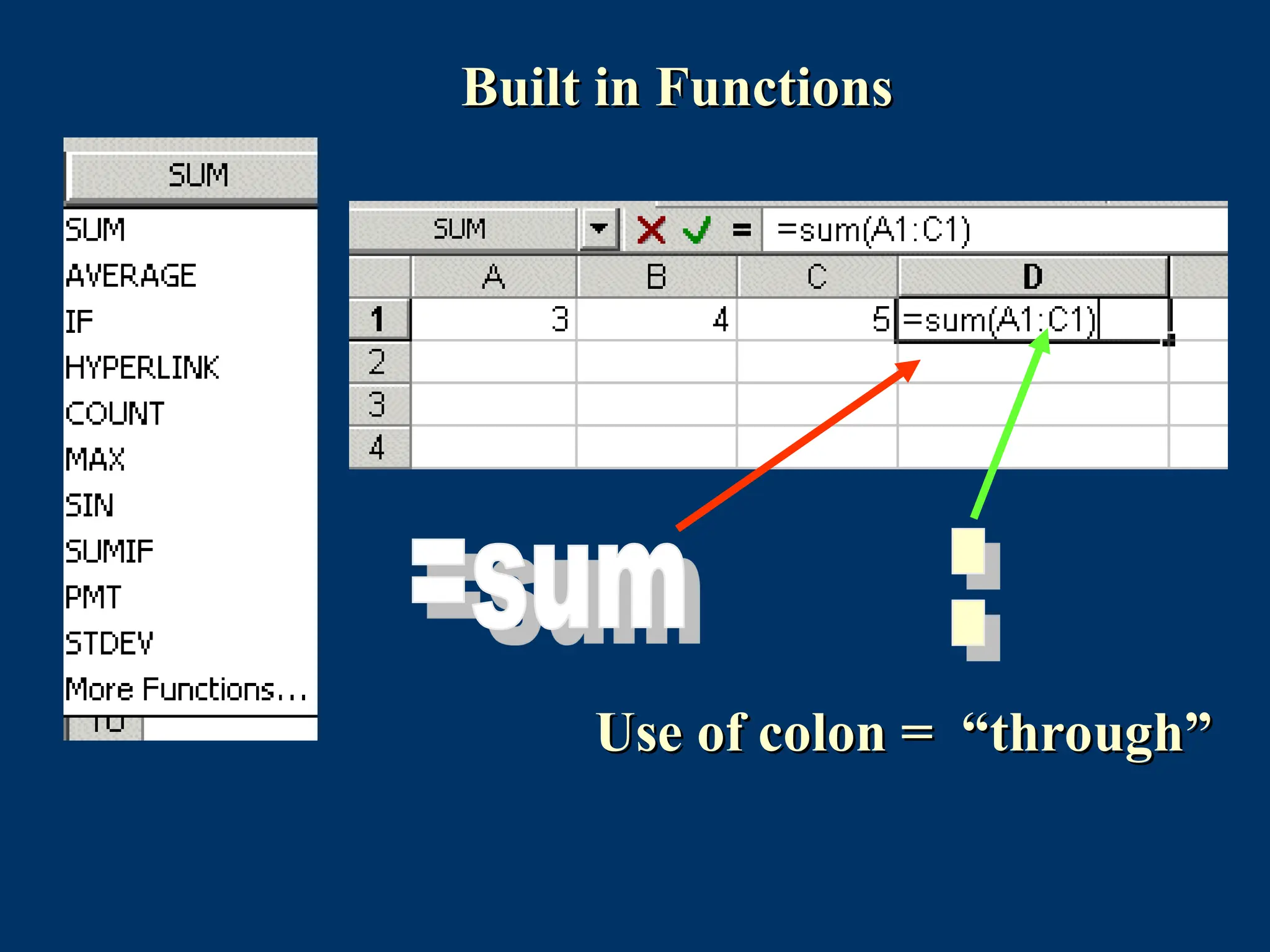
6. Input a formula for adding and averaging data.

3. What is a Spreadsheet?
A program that allows you to use data to
forecast, manage, predict, and present
information.

4. Spreadsheet Uses
Spreadsheet Uses
School:
School: Student grades, payroll
Sports:
Sports: individual and team statistics
Personal:
Personal: checkbook, household expenses
Business:
Business: payroll, investments

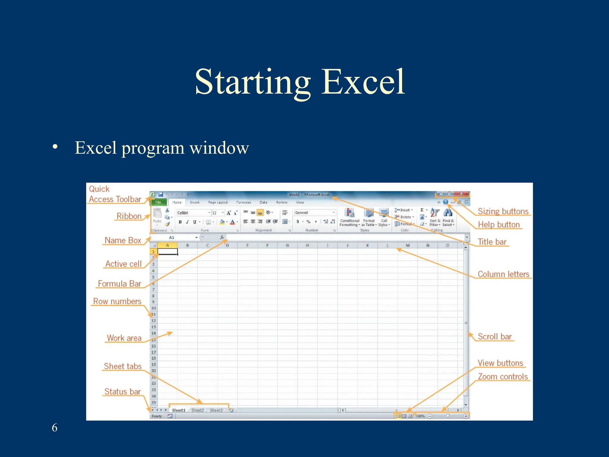
5. Introduction to Excel
• columns – identified with alphabetic headings
• rows - identified with numeric headings
• and their intersections are called cells
• (Cell references: B4, A20)
Spreadsheets are made up of :

6. Starting Excel
• Excel program window
6

7. Introduction to Excel
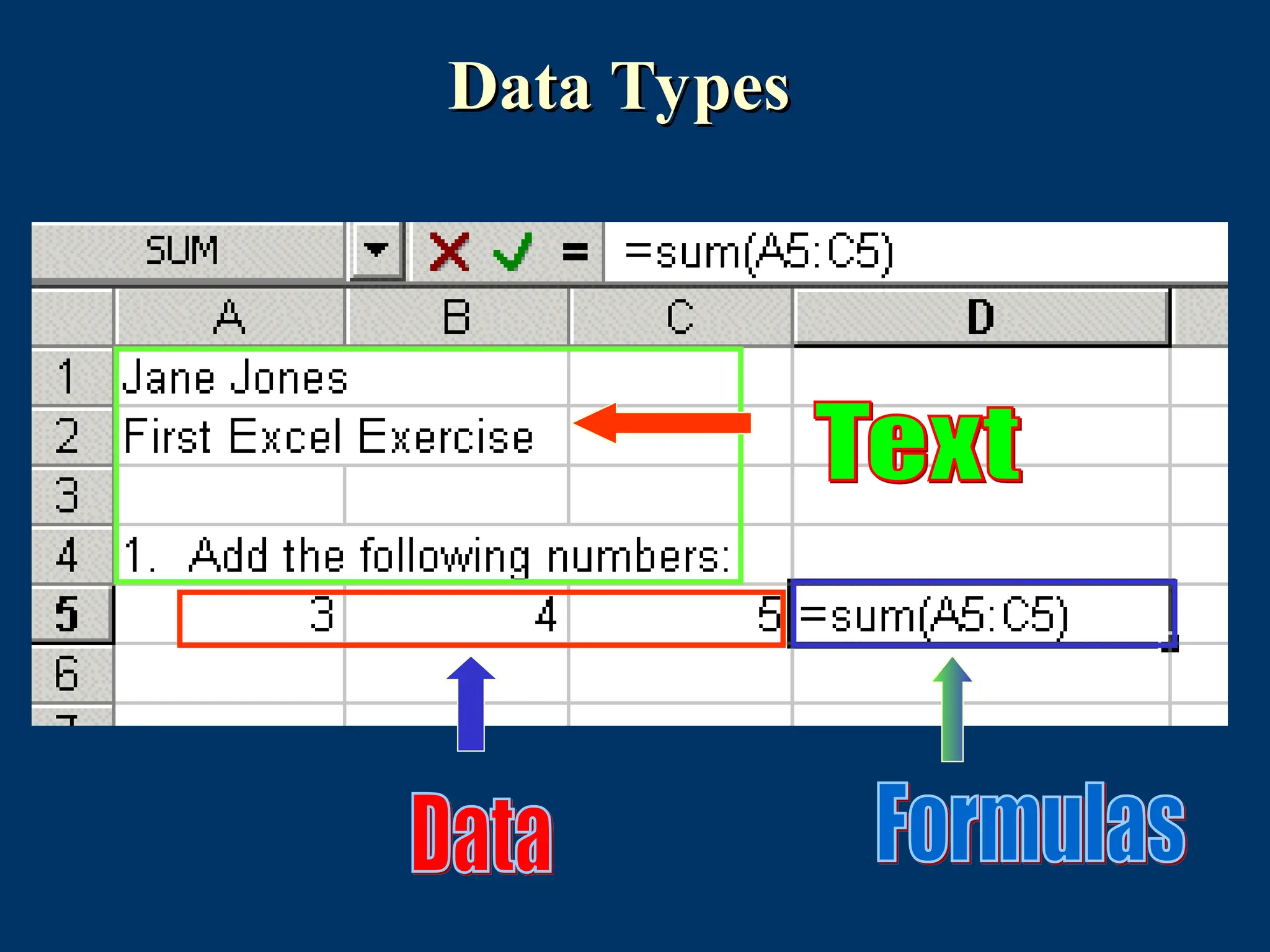
In each cell there may be the following types of data
• text (labels)
• number data (constants)
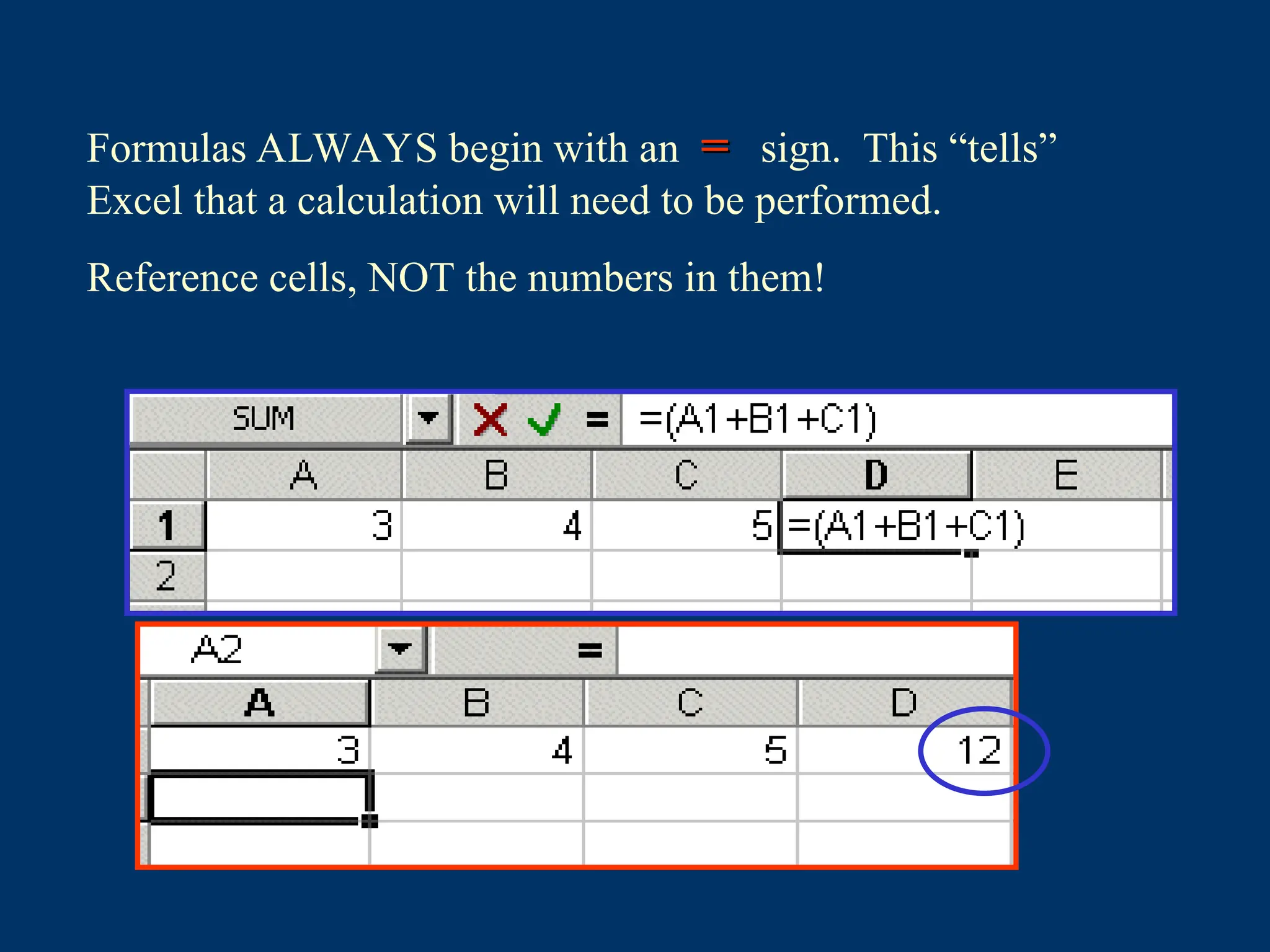
• formulas (mathematical equations that do all the work)

8. Data Types
Data Types

9. Formulas ALWAYS begin with an =
= sign. This “tells”
Excel that a calculation will need to be performed.
Reference cells, NOT the numbers in them!

10. Built in Functions
Built in Functions
Use of colon = “through”
Use of colon = “through”

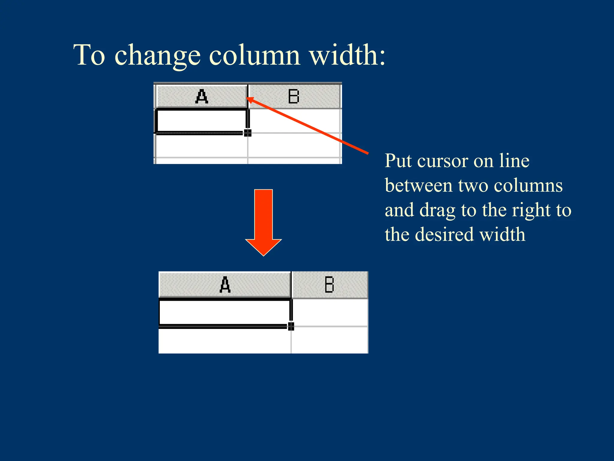
11. To change column width:
Put cursor on line
between two columns
and drag to the right to
the desired width

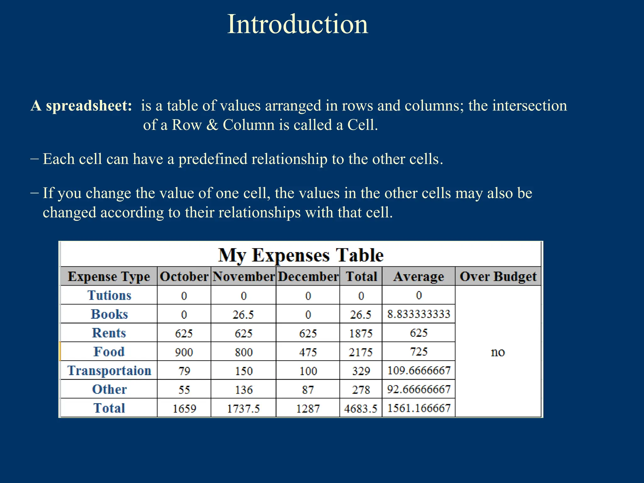
12. A spreadsheet: is a table of values arranged in rows and columns; the intersection
of a Row & Column is called a Cell.
– Each cell can have a predefined relationship to the other cells.
– If you change the value of one cell, the values in the other cells may also be
changed according to their relationships with that cell.
Introduction

13. Introduction
• Excel is the MS-Office Application program used for creating
spreadsheets.
• You can use Excel to enter all sorts of data and perform financial,
mathematical, or statistical calculations.
• Excel operates like other MS Office programs and has many of the
same functions and shortcuts as MS Word & MS PowerPoint.
• Excel can do most (not all) of the common (i.e. useful & popular)
tasks done in MATLAB or similar software.
• MATLAB is more powerful, but it’s also SPECIALIZED and
EXPENSIVE.
• Excel is more widespread, quick, and easy.

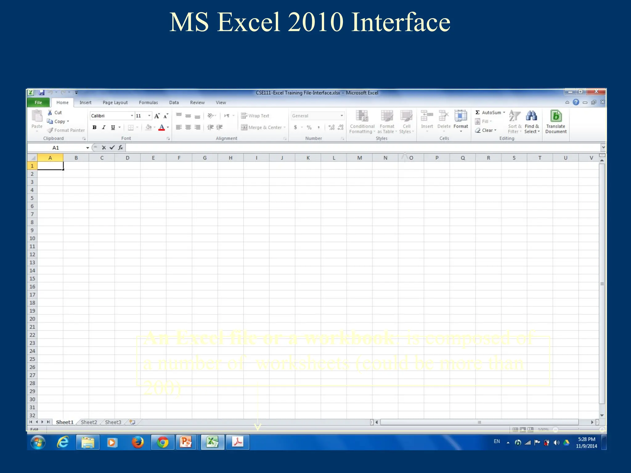
14. MS Excel 2010 Interface
An Excel file or a workbook: is composed of
a number of worksheets (could be more than
200)

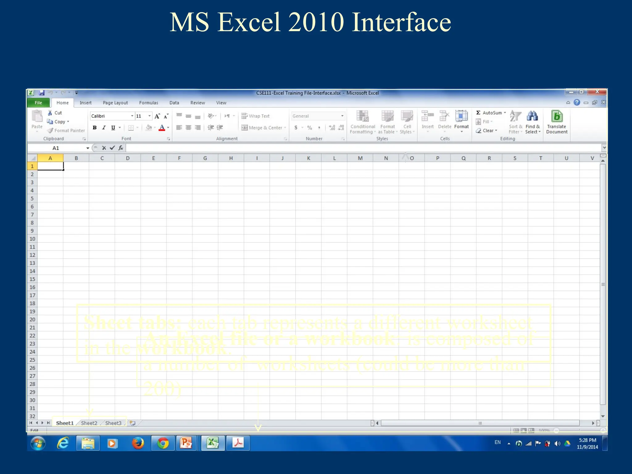
15. MS Excel 2010 Interface
An Excel file or a workbook: is composed of
a number of worksheets (could be more than
200)
Sheet tabs: each tab represents a different worksheet
in the workbook.

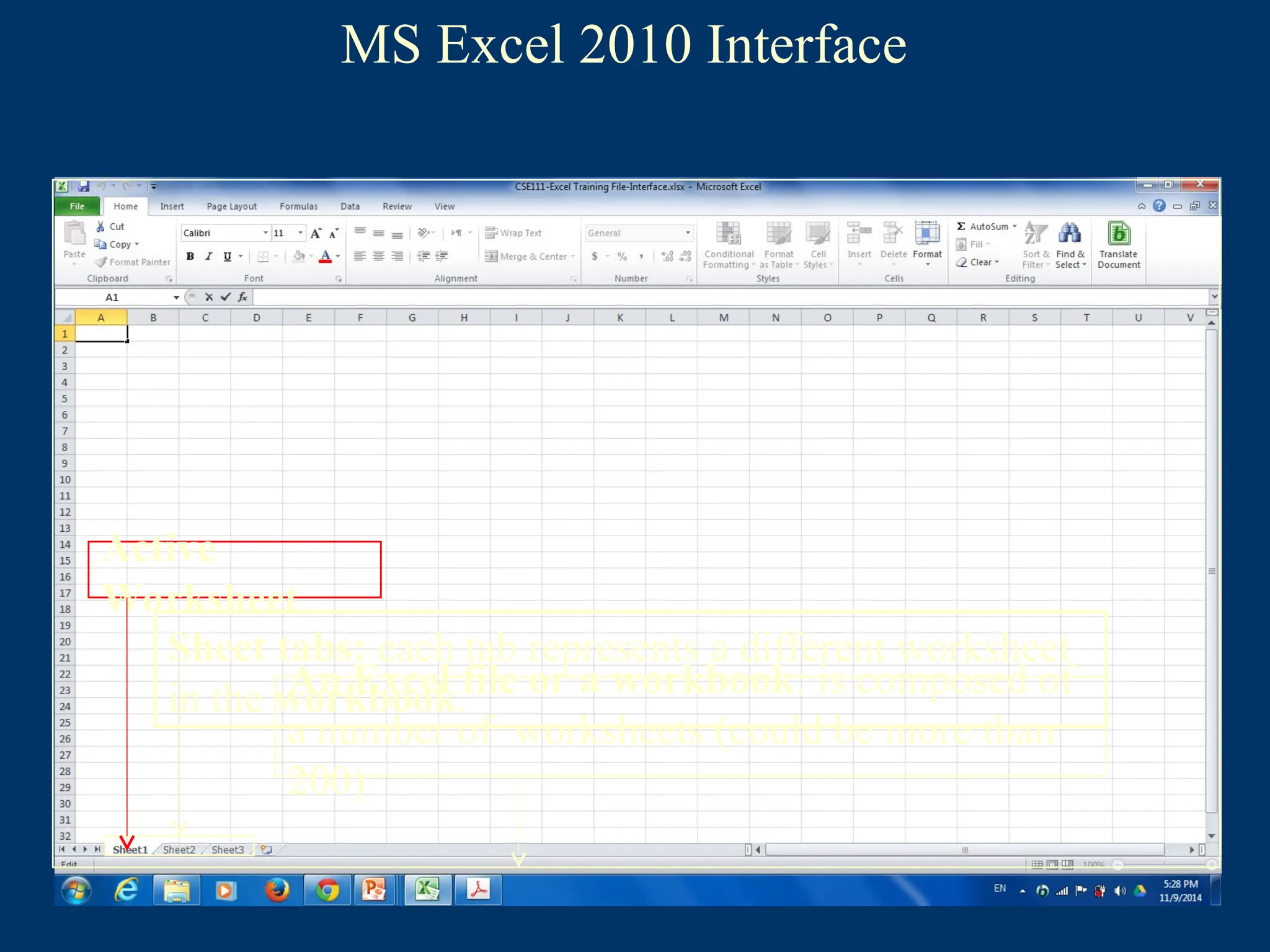
16. MS Excel 2010 Interface
An Excel file or a workbook: is composed of
a number of worksheets (could be more than
200)
Sheet tabs: each tab represents a different worksheet
in the workbook.
Active
Worksheet

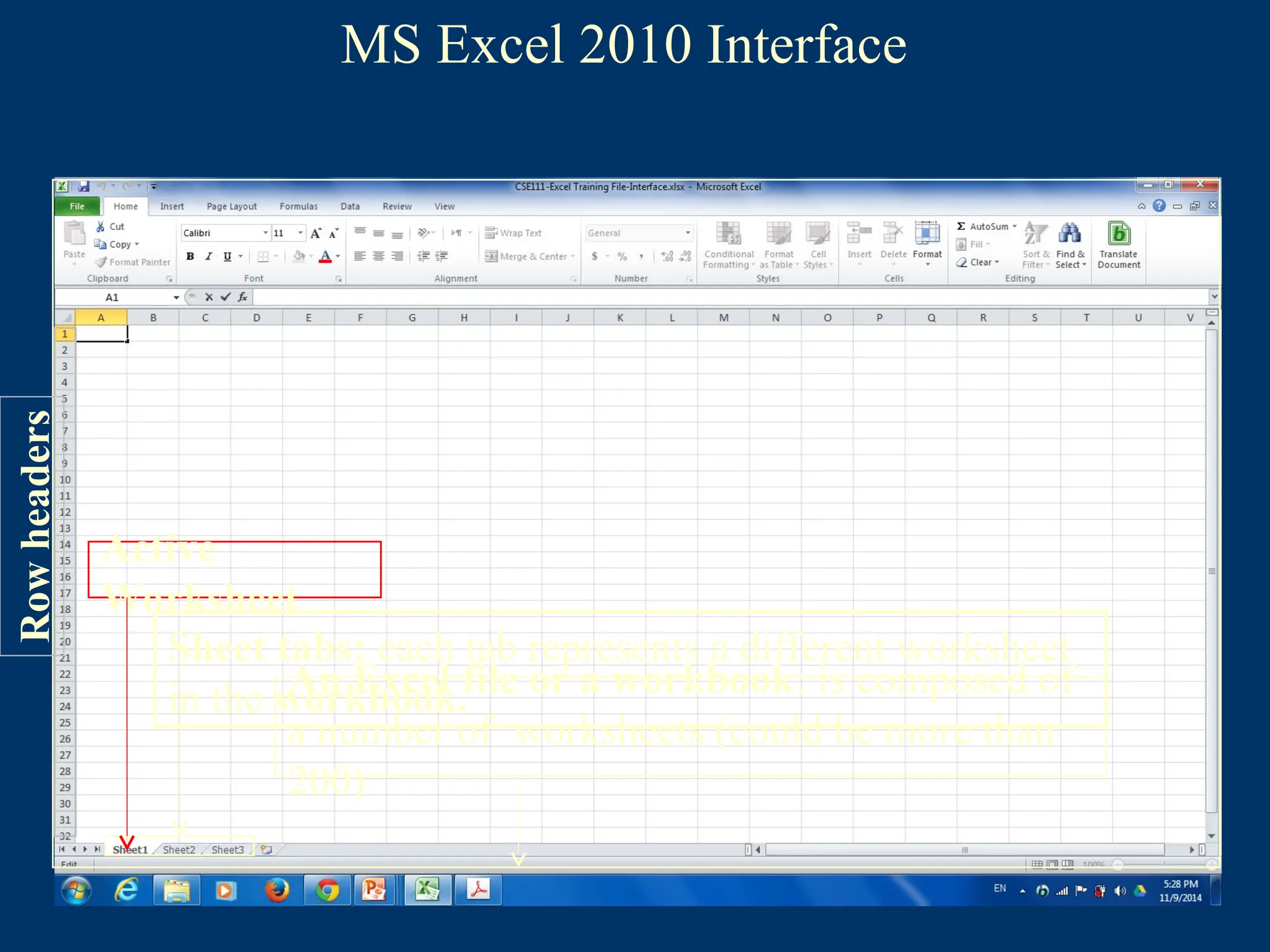
17. MS Excel 2010 Interface
An Excel file or a workbook: is composed of
a number of worksheets (could be more than
200)
Sheet tabs: each tab represents a different worksheet
in the workbook.
Active
Worksheet
Row
headers

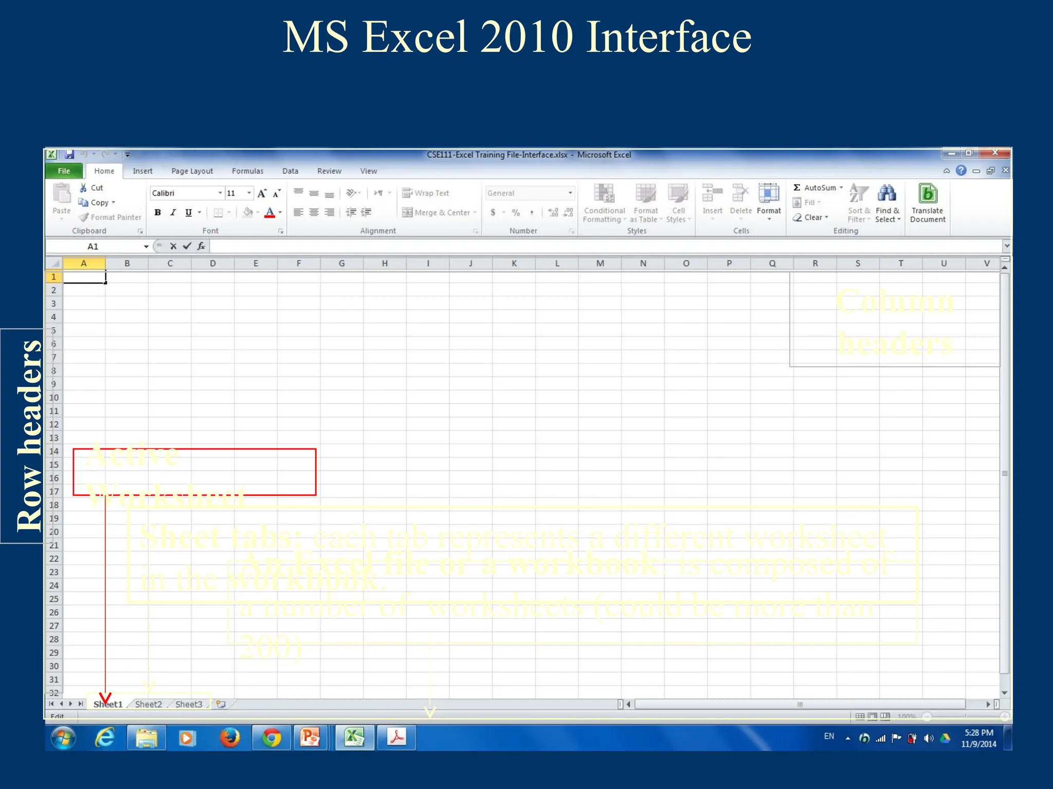
18. MS Excel 2010 Interface
An Excel file or a workbook: is composed of
a number of worksheets (could be more than
200)
Sheet tabs: each tab represents a different worksheet
in the workbook.
Active
Worksheet
Row
headers
Column
headers

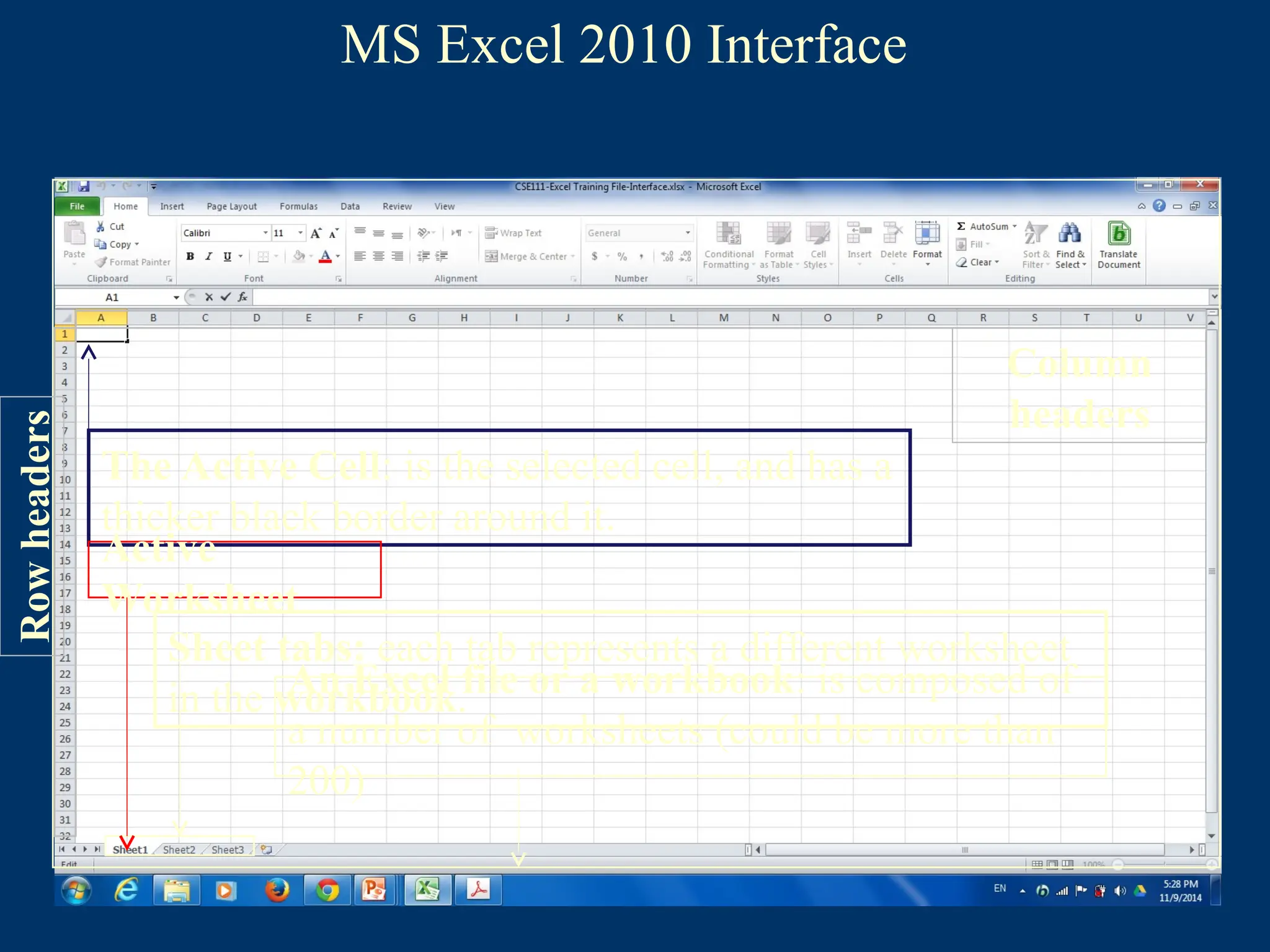
19. MS Excel 2010 Interface
An Excel file or a workbook: is composed of
a number of worksheets (could be more than
200)
Sheet tabs: each tab represents a different worksheet
in the workbook.
The Active Cell: is the selected cell, and has a
thicker black border around it.
Active
Worksheet
Row
headers
Column
headers

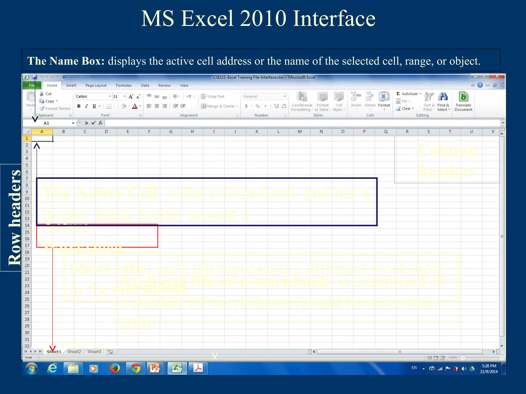
20. MS Excel 2010 Interface
The Name Box: displays the active cell address or the name of the selected cell, range, or object.
An Excel file or a workbook: is composed of
a number of worksheets (could be more than
200)
Sheet tabs: each tab represents a different worksheet
in the workbook.
Active
Worksheet
The Active Cell: is the selected cell, and has a
thicker black border around it.
Row
headers
Column
headers

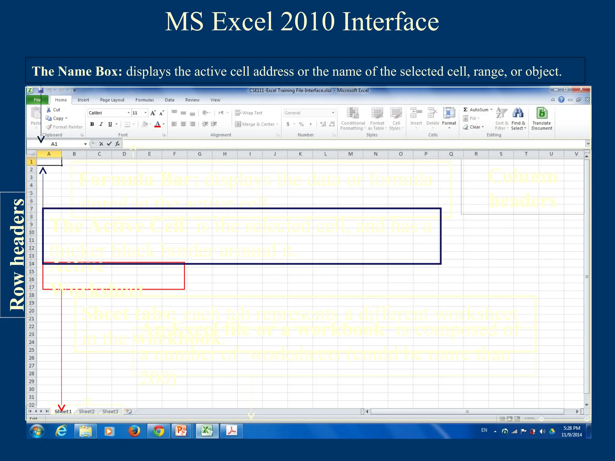
21. MS Excel 2010 Interface
The Name Box: displays the active cell address or the name of the selected cell, range, or object.
Formula Bar: displays the data or formula
stored in the active cell.
An Excel file or a workbook: is composed of
a number of worksheets (could be more than
200)
Sheet tabs: each tab represents a different worksheet
in the workbook.
Active
Worksheet
The Active Cell: is the selected cell, and has a
thicker black border around it.
Row
headers
Row
headers
Column
headers

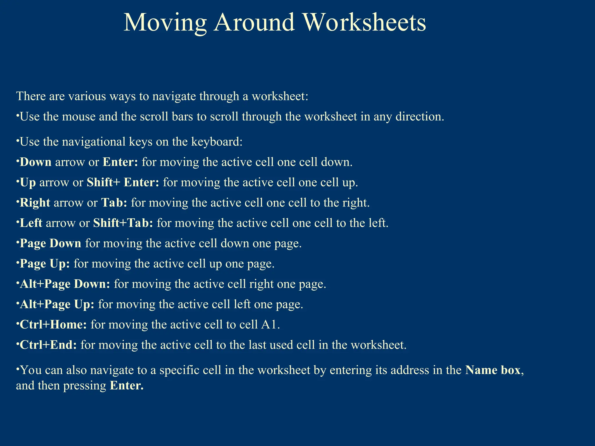
22. There are various ways to navigate through a worksheet:
•Use the mouse and the scroll bars to scroll through the worksheet in any direction.
•Use the navigational keys on the keyboard:
•Down arrow or Enter: for moving the active cell one cell down.
•Up arrow or Shift+ Enter: for moving the active cell one cell up.
•Right arrow or Tab: for moving the active cell one cell to the right.
•Left arrow or Shift+Tab: for moving the active cell one cell to the left.
•Page Down for moving the active cell down one page.
•Page Up: for moving the active cell up one page.
•Alt+Page Down: for moving the active cell right one page.
•Alt+Page Up: for moving the active cell left one page.
•Ctrl+Home: for moving the active cell to cell A1.
•Ctrl+End: for moving the active cell to the last used cell in the worksheet.
•You can also navigate to a specific cell in the worksheet by entering its address in the Name box,
and then pressing Enter.
Moving Around Worksheets

23. Selecting Cells, Rows, and Columns
• To select a single cell, just click on it.

24. Selecting Cells, Rows, and Columns
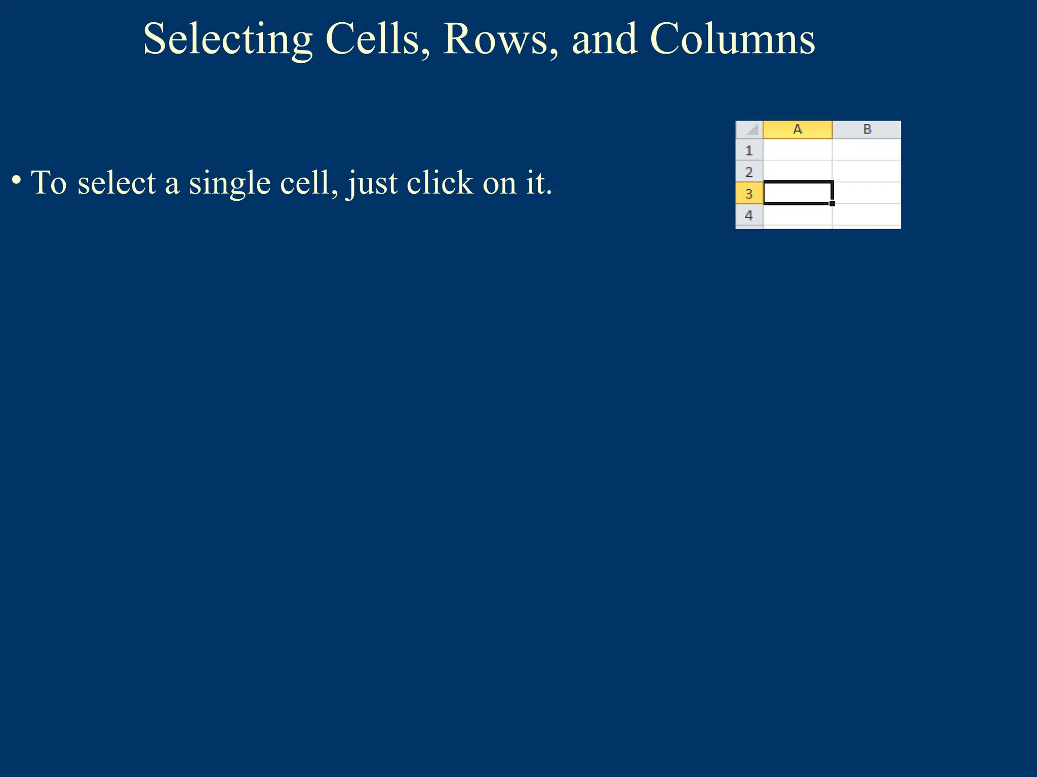
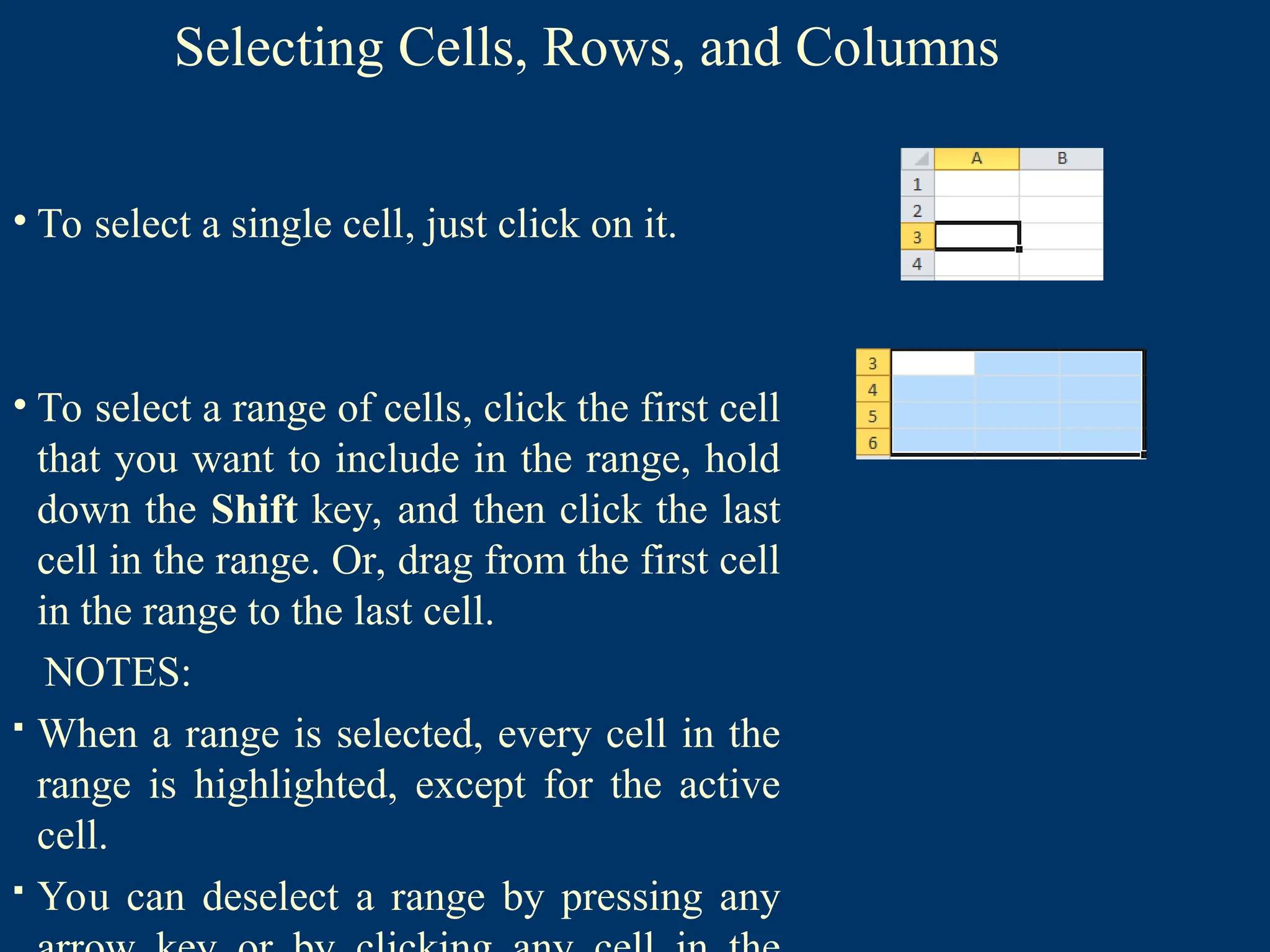
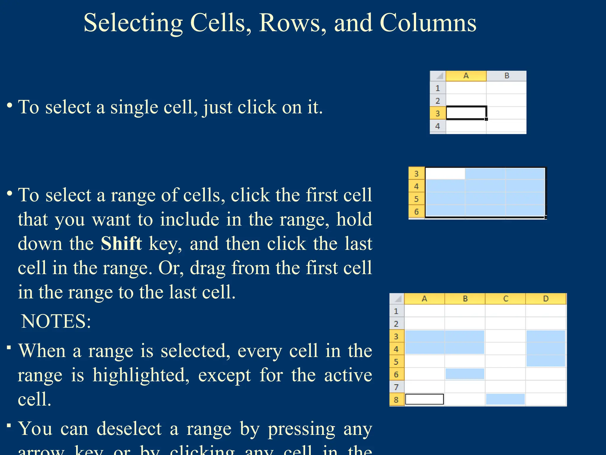
• To select a single cell, just click on it.
• To select a range of cells, click the first cell
that you want to include in the range, hold
down the Shift key, and then click the last
cell in the range. Or, drag from the first cell
in the range to the last cell.
NOTES:
 When a range is selected, every cell in the
range is highlighted, except for the active
cell.
 You can deselect a range by pressing any

25. Selecting Cells, Rows, and Columns
• To select a single cell, just click on it.
• To select a range of cells, click the first cell
that you want to include in the range, hold
down the Shift key, and then click the last
cell in the range. Or, drag from the first cell
in the range to the last cell.
NOTES:
 When a range is selected, every cell in the
range is highlighted, except for the active
cell.
 You can deselect a range by pressing any

26. Selecting Cells, Rows, and Columns
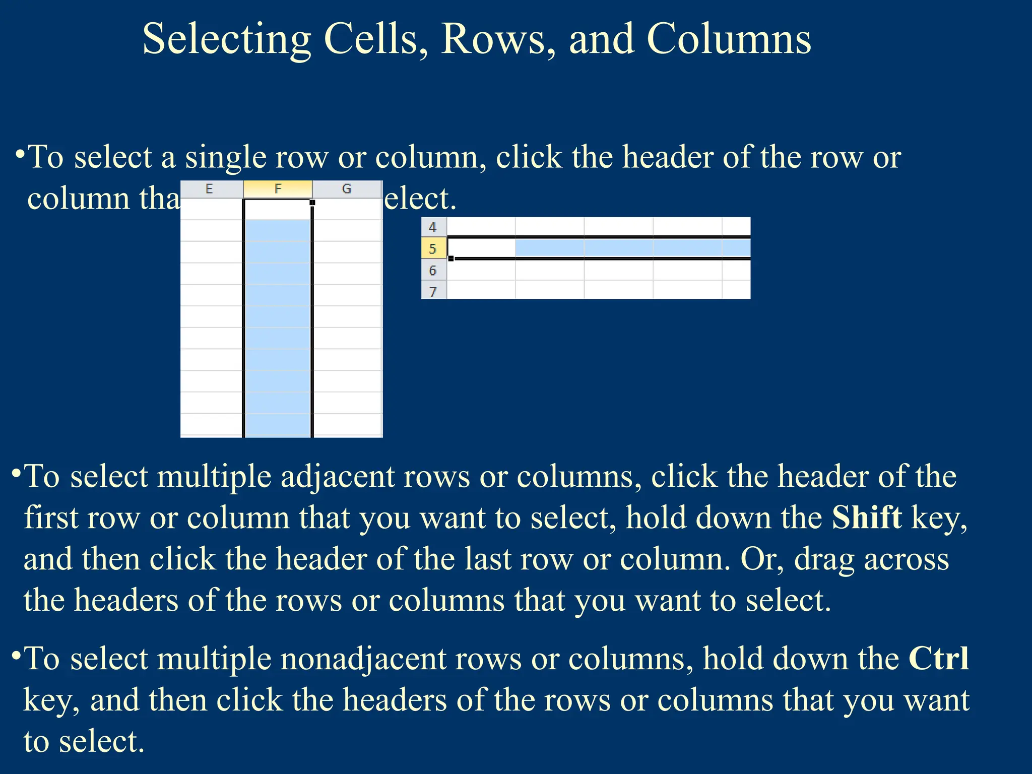
•To select a single row or column, click the header of the row or
column that you want to select.
•To select multiple adjacent rows or columns, click the header of the
first row or column that you want to select, hold down the Shift key,
and then click the header of the last row or column. Or, drag across
the headers of the rows or columns that you want to select.
•To select multiple nonadjacent rows or columns, hold down the Ctrl
key, and then click the headers of the rows or columns that you want
to select.

27. Editing & Formatting Worksheets
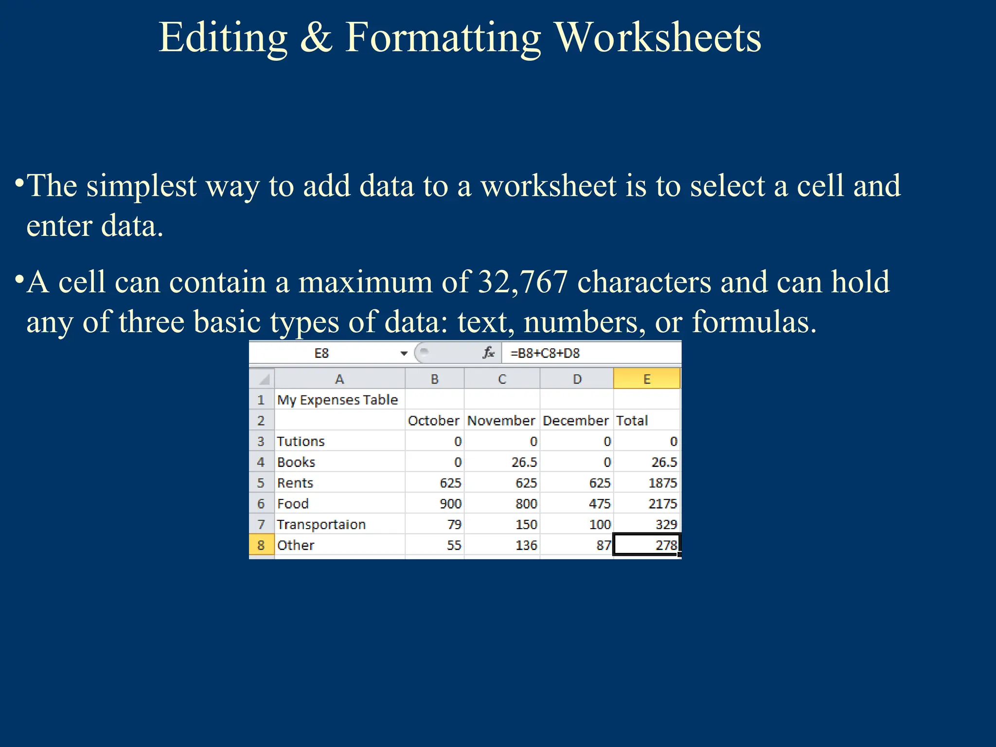
•The simplest way to add data to a worksheet is to select a cell and
enter data.
•A cell can contain a maximum of 32,767 characters and can hold
any of three basic types of data: text, numbers, or formulas.

28. Editing & Formatting Worksheets
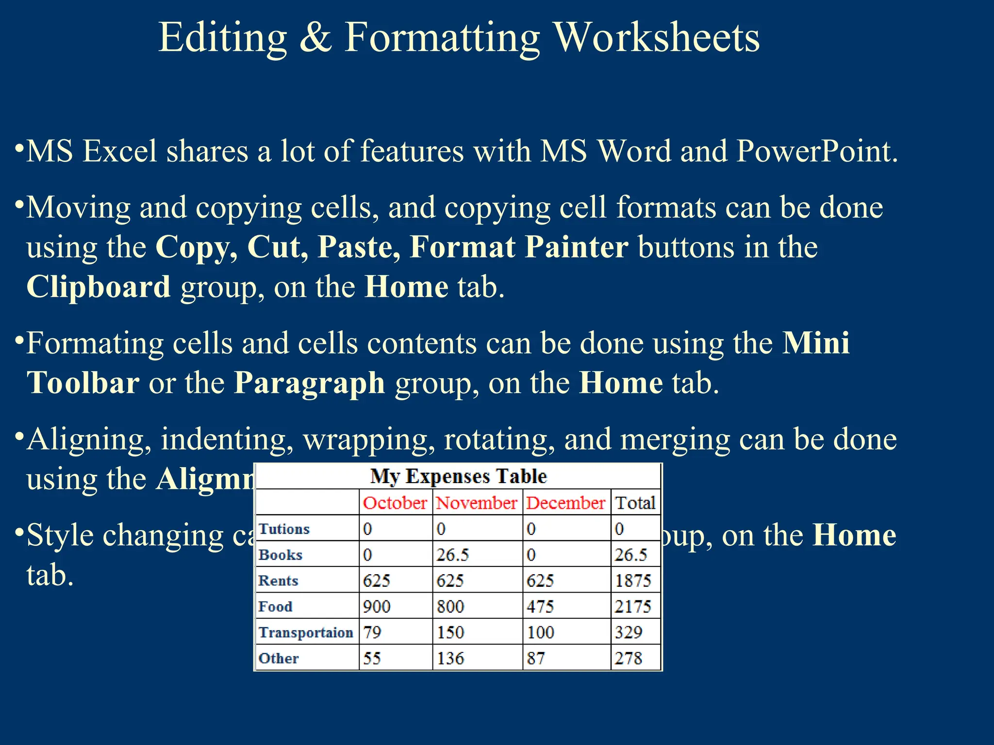
•MS Excel shares a lot of features with MS Word and PowerPoint.
•Moving and copying cells, and copying cell formats can be done
using the Copy, Cut, Paste, Format Painter buttons in the
Clipboard group, on the Home tab.
•Formating cells and cells contents can be done using the Mini
Toolbar or the Paragraph group, on the Home tab.
•Aligning, indenting, wrapping, rotating, and merging can be done
using the Aligmnet group, on the Home tab.
•Style changing can be done, using the Styles group, on the Home
tab.

29. Formatting Numbers
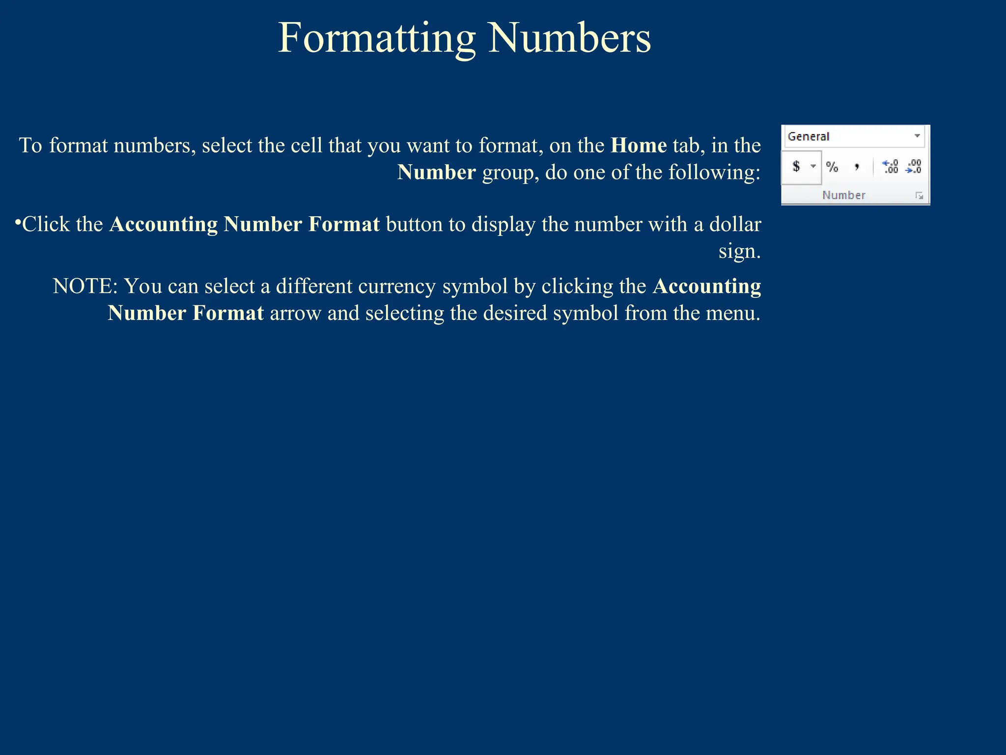
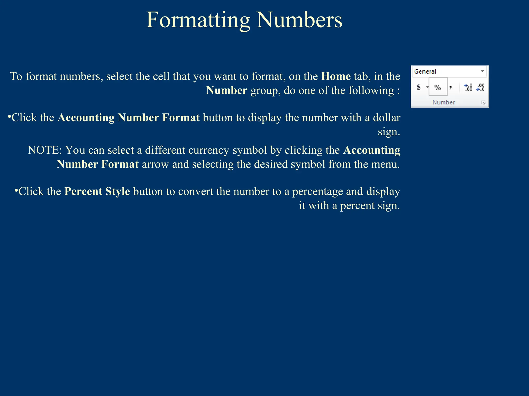
To format numbers, select the cell that you want to format, on the Home tab, in the
Number group, do one of the following:
•Click the Accounting Number Format button to display the number with a dollar
sign.
NOTE: You can select a different currency symbol by clicking the Accounting
Number Format arrow and selecting the desired symbol from the menu.

30. Formatting Numbers
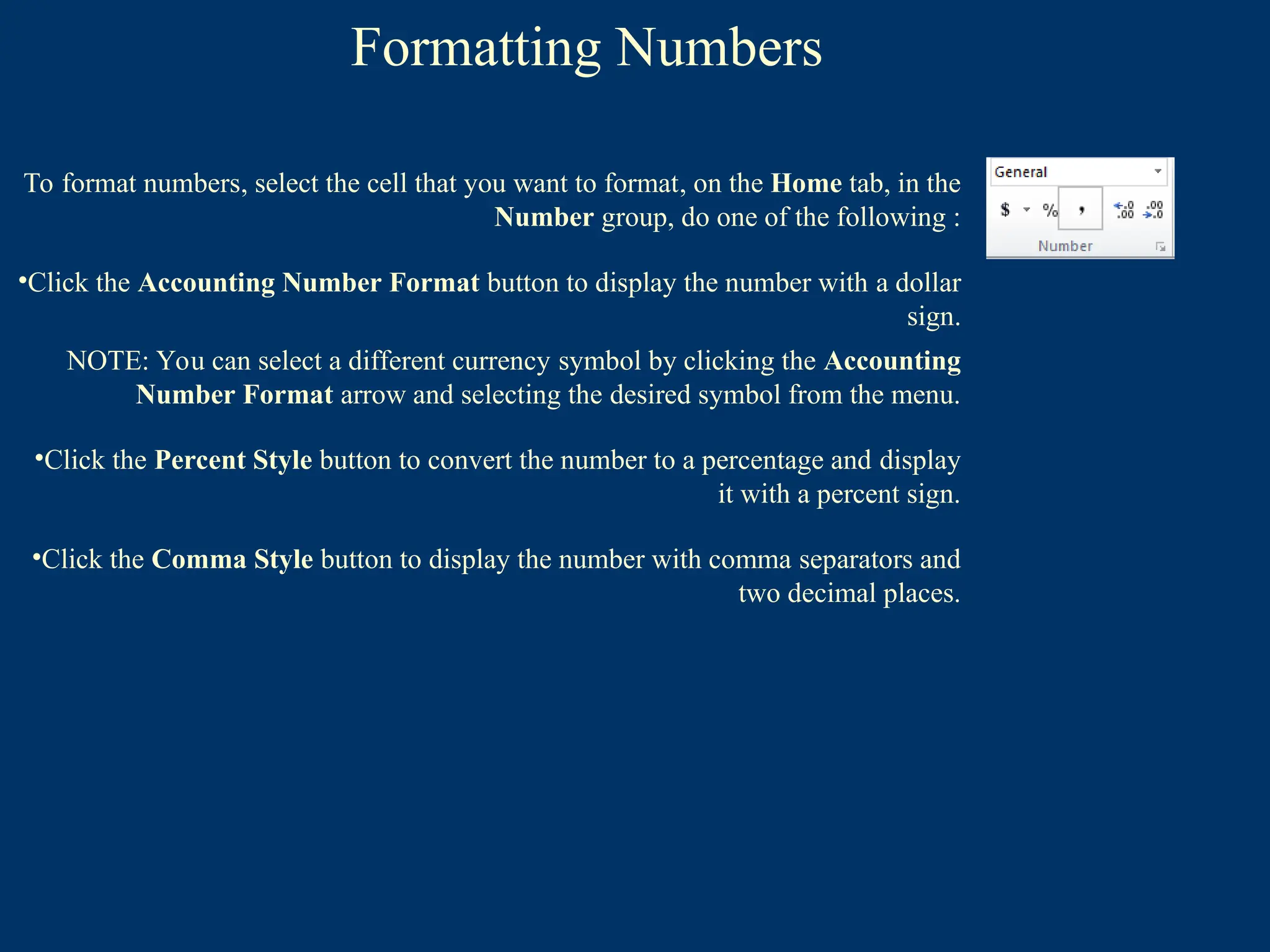
To format numbers, select the cell that you want to format, on the Home tab, in the
Number group, do one of the following :
•Click the Accounting Number Format button to display the number with a dollar
sign.
NOTE: You can select a different currency symbol by clicking the Accounting
Number Format arrow and selecting the desired symbol from the menu.
•Click the Percent Style button to convert the number to a percentage and display
it with a percent sign.

31. Formatting Numbers
To format numbers, select the cell that you want to format, on the Home tab, in the
Number group, do one of the following :
•Click the Accounting Number Format button to display the number with a dollar
sign.
NOTE: You can select a different currency symbol by clicking the Accounting
Number Format arrow and selecting the desired symbol from the menu.
•Click the Percent Style button to convert the number to a percentage and display
it with a percent sign.
•Click the Comma Style button to display the number with comma separators and
two decimal places.

32. Formatting Numbers
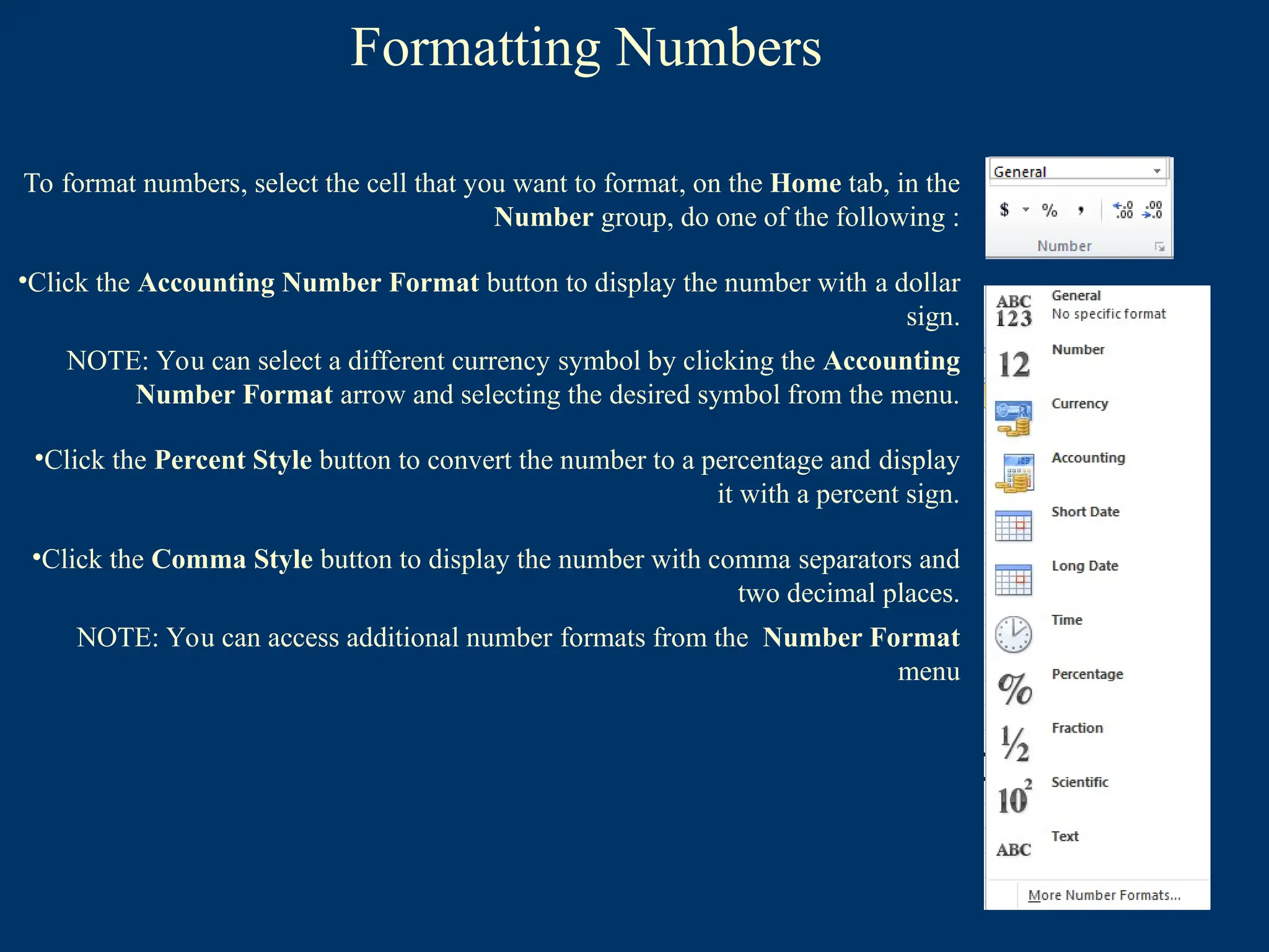
To format numbers, select the cell that you want to format, on the Home tab, in the
Number group, do one of the following :
•Click the Accounting Number Format button to display the number with a dollar
sign.
NOTE: You can select a different currency symbol by clicking the Accounting
Number Format arrow and selecting the desired symbol from the menu.
•Click the Percent Style button to convert the number to a percentage and display
it with a percent sign.
•Click the Comma Style button to display the number with comma separators and
two decimal places.
NOTE: You can access additional number formats from the Number Format
menu

33. Formatting Numbers
To format numbers, select the cell that you want to format, on the Home tab, in the
Number group, do one of the following :
•Click the Accounting Number Format button to display the number with a dollar
sign.
NOTE: You can select a different currency symbol by clicking the Accounting
Number Format arrow and selecting the desired symbol from the menu.
•Click the Percent Style button to convert the number to a percentage and display
it with a percent sign.
•Click the Comma Style button to display the number with comma separators and
two decimal places.
NOTE: You can access additional number formats from the Number Format
menu
To change the number of decimal places, select the cell that you want to format,
and then on the Home tab, in the Number group, do one of the following:
•Click the Increase Decimal button to increase the number of decimal places.
•Click the Decrease Decimal button to decrease the number of decimal places.

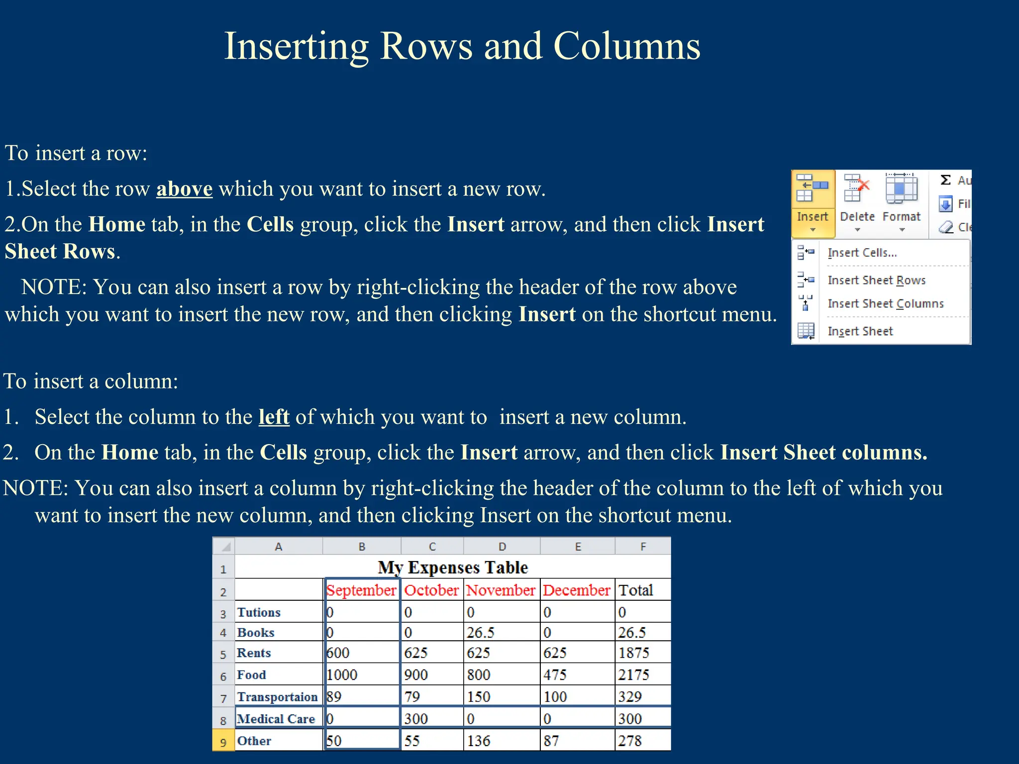
34. Inserting Rows and Columns
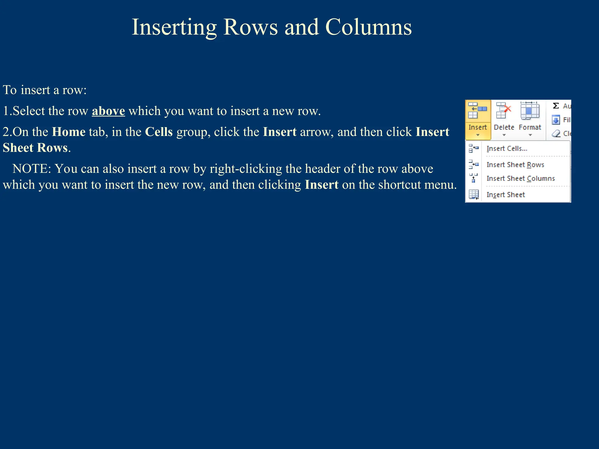
To insert a row:
1.Select the row above which you want to insert a new row.
2.On the Home tab, in the Cells group, click the Insert arrow, and then click Insert
Sheet Rows.
NOTE: You can also insert a row by right-clicking the header of the row above
which you want to insert the new row, and then clicking Insert on the shortcut menu.

35. Inserting Rows and Columns
To insert a column:
1. Select the column to the left of which you want to insert a new column.
2. On the Home tab, in the Cells group, click the Insert arrow, and then click Insert Sheet columns.
NOTE: You can also insert a column by right-clicking the header of the column to the left of which you
want to insert the new column, and then clicking Insert on the shortcut menu.
To insert a row:
1.Select the row above which you want to insert a new row.
2.On the Home tab, in the Cells group, click the Insert arrow, and then click Insert
Sheet Rows.
NOTE: You can also insert a row by right-clicking the header of the row above
which you want to insert the new row, and then clicking Insert on the shortcut menu.

36. Inserting Rows and Columns
To insert a column:
1. Select the column to the left of which you want to insert a new column.
2. On the Home tab, in the Cells group, click the Insert arrow, and then click Insert Sheet columns.
NOTE: You can also insert a column by right-clicking the header of the column to the left of which you
want to insert the new column, and then clicking Insert on the shortcut menu.
To insert a row:
1.Select the row above which you want to insert a new row.
2.On the Home tab, in the Cells group, click the Insert arrow, and then click Insert
Sheet Rows.
NOTE: You can also insert a row by right-clicking the header of the row above
which you want to insert the new row, and then clicking Insert on the shortcut menu.

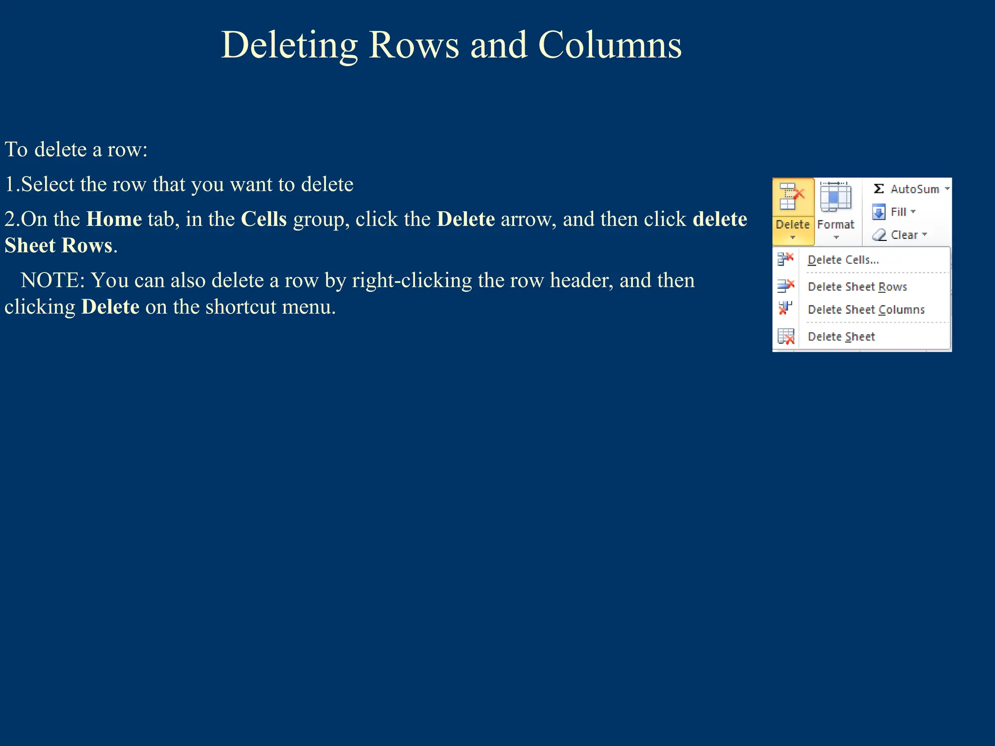
37. Deleting Rows and Columns
To delete a row:
1.Select the row that you want to delete
2.On the Home tab, in the Cells group, click the Delete arrow, and then click delete
Sheet Rows.
NOTE: You can also delete a row by right-clicking the row header, and then
clicking Delete on the shortcut menu.

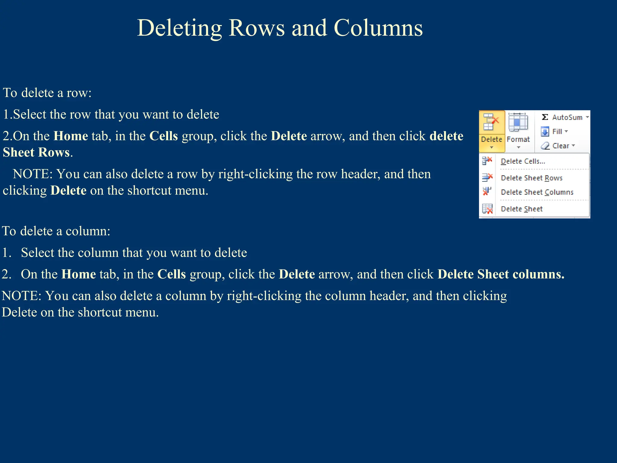
38. Deleting Rows and Columns
To delete a column:
1. Select the column that you want to delete
2. On the Home tab, in the Cells group, click the Delete arrow, and then click Delete Sheet columns.
NOTE: You can also delete a column by right-clicking the column header, and then clicking
Delete on the shortcut menu.
To delete a row:
1.Select the row that you want to delete
2.On the Home tab, in the Cells group, click the Delete arrow, and then click delete
Sheet Rows.
NOTE: You can also delete a row by right-clicking the row header, and then
clicking Delete on the shortcut menu.

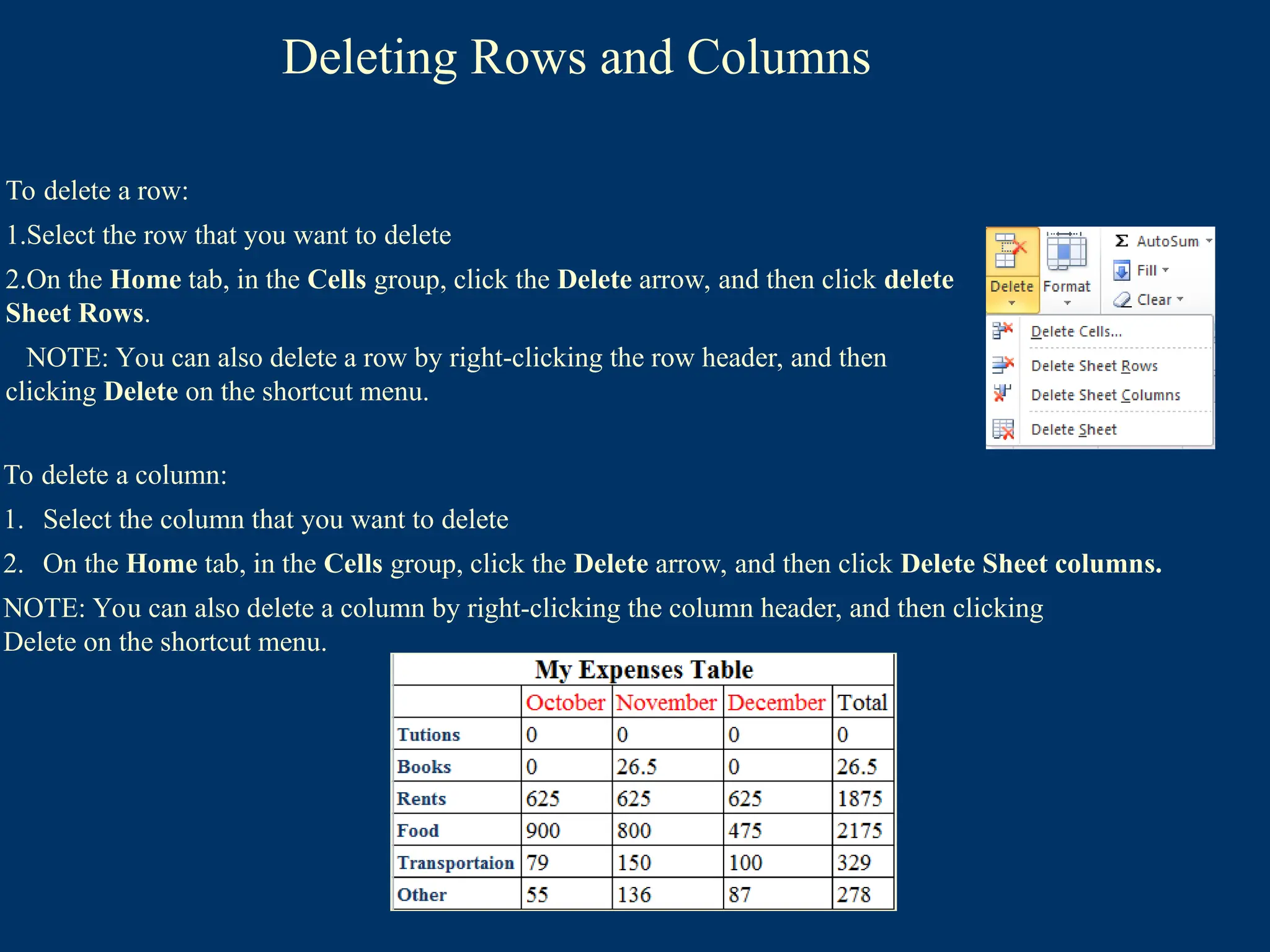
39. Deleting Rows and Columns
To delete a column:
1. Select the column that you want to delete
2. On the Home tab, in the Cells group, click the Delete arrow, and then click Delete Sheet columns.
NOTE: You can also delete a column by right-clicking the column header, and then clicking
Delete on the shortcut menu.
To delete a row:
1.Select the row that you want to delete
2.On the Home tab, in the Cells group, click the Delete arrow, and then click delete
Sheet Rows.
NOTE: You can also delete a row by right-clicking the row header, and then
clicking Delete on the shortcut menu.

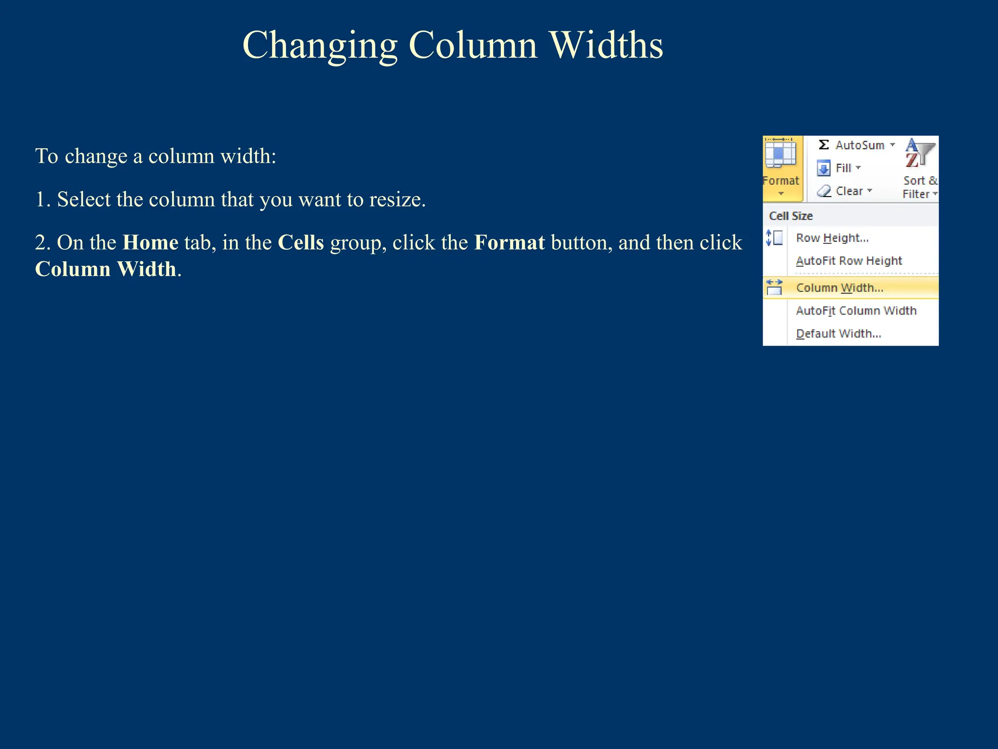
40. Changing Column Widths
To change a column width:
1. Select the column that you want to resize.
2. On the Home tab, in the Cells group, click the Format button, and then click
Column Width.

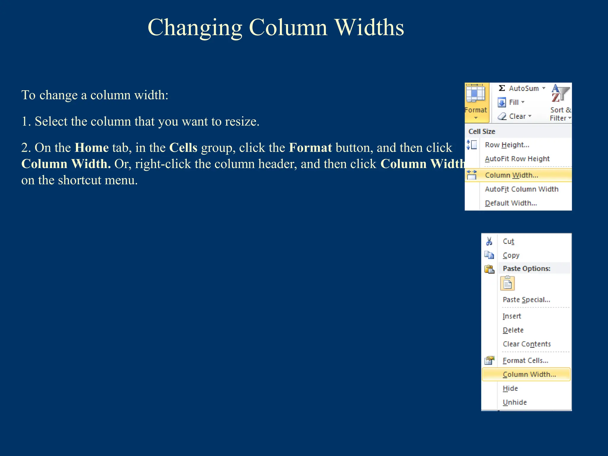
41. Changing Column Widths
To change a column width:
1. Select the column that you want to resize.
2. On the Home tab, in the Cells group, click the Format button, and then click
Column Width. Or, right-click the column header, and then click Column Width
on the shortcut menu.

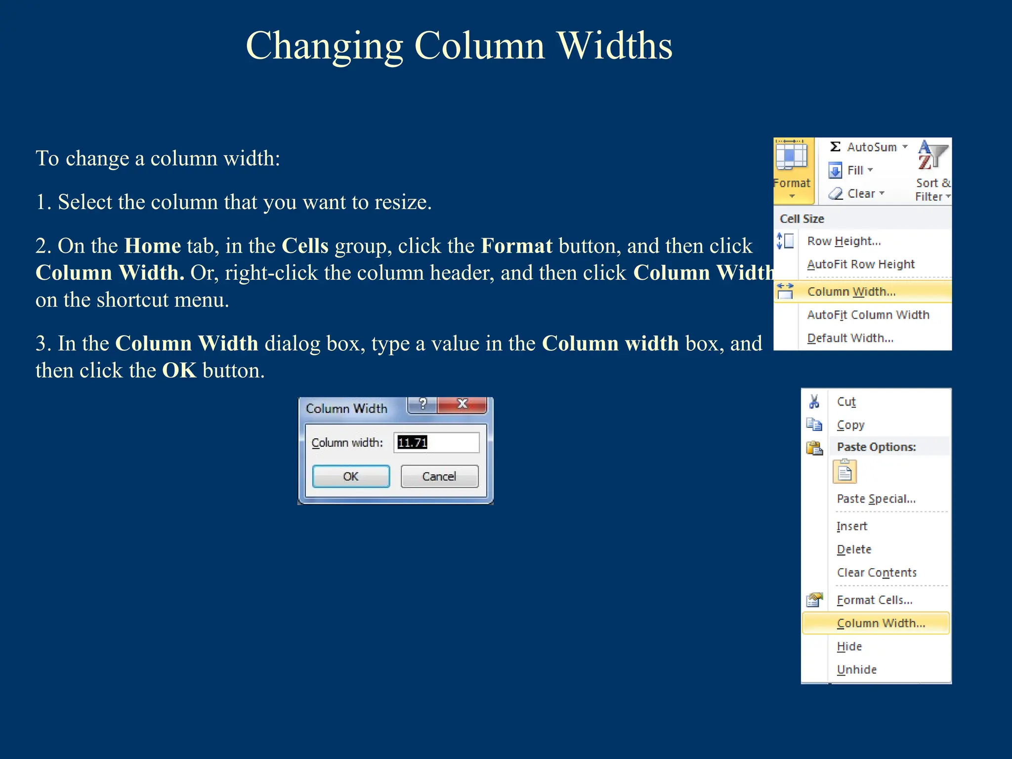
42. Changing Column Widths
To change a column width:
1. Select the column that you want to resize.
2. On the Home tab, in the Cells group, click the Format button, and then click
Column Width. Or, right-click the column header, and then click Column Width
on the shortcut menu.
3. In the Column Width dialog box, type a value in the Column width box, and
then click the OK button.

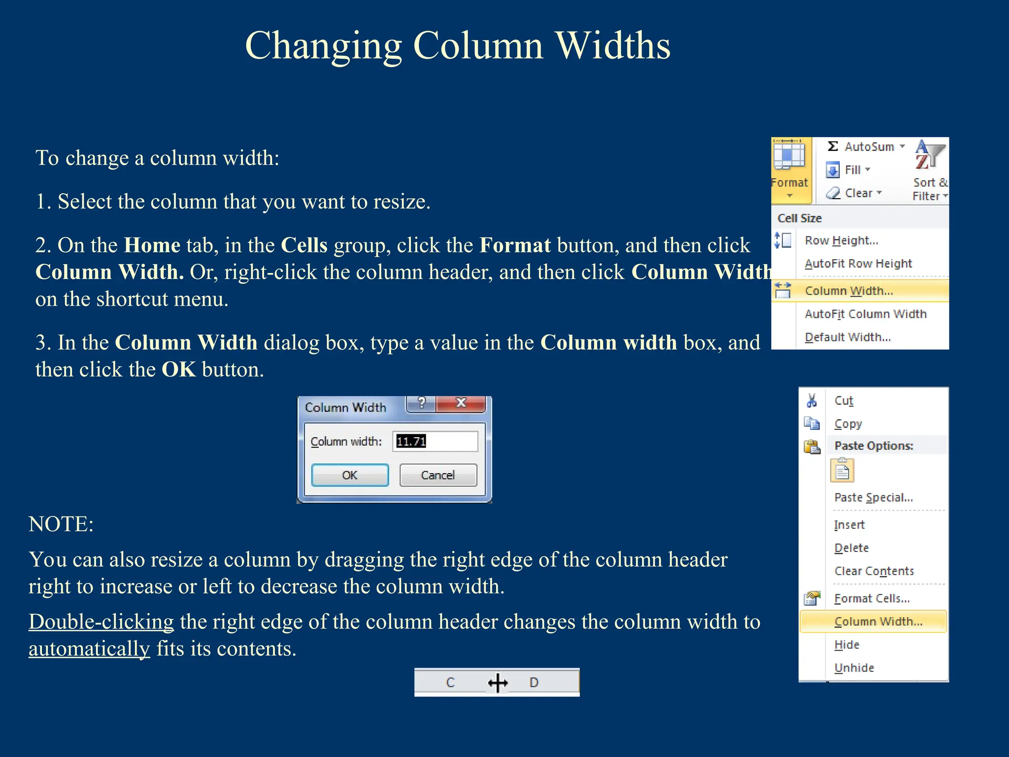
43. Changing Column Widths
To change a column width:
1. Select the column that you want to resize.
2. On the Home tab, in the Cells group, click the Format button, and then click
Column Width. Or, right-click the column header, and then click Column Width
on the shortcut menu.
3. In the Column Width dialog box, type a value in the Column width box, and
then click the OK button.
NOTE:
You can also resize a column by dragging the right edge of the column header
right to increase or left to decrease the column width.
Double-clicking the right edge of the column header changes the column width to
automatically fits its contents.

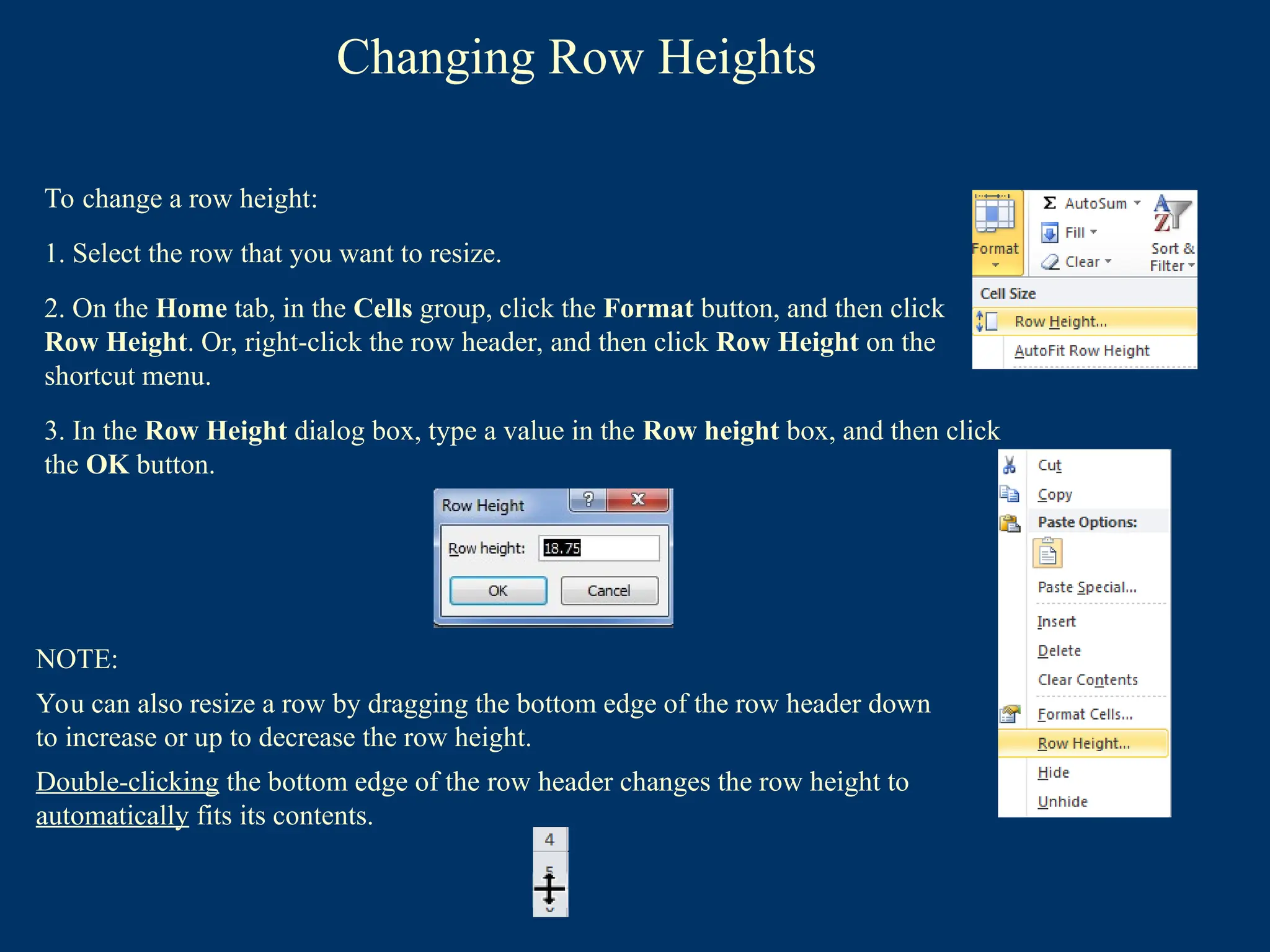
44. Changing Row Heights
To change a row height:
1. Select the row that you want to resize.
2. On the Home tab, in the Cells group, click the Format button, and then click
Row Height. Or, right-click the row header, and then click Row Height on the
shortcut menu.
3. In the Row Height dialog box, type a value in the Row height box, and then click
the OK button.
NOTE:
You can also resize a row by dragging the bottom edge of the row header down
to increase or up to decrease the row height.
Double-clicking the bottom edge of the row header changes the row height to
automatically fits its contents.

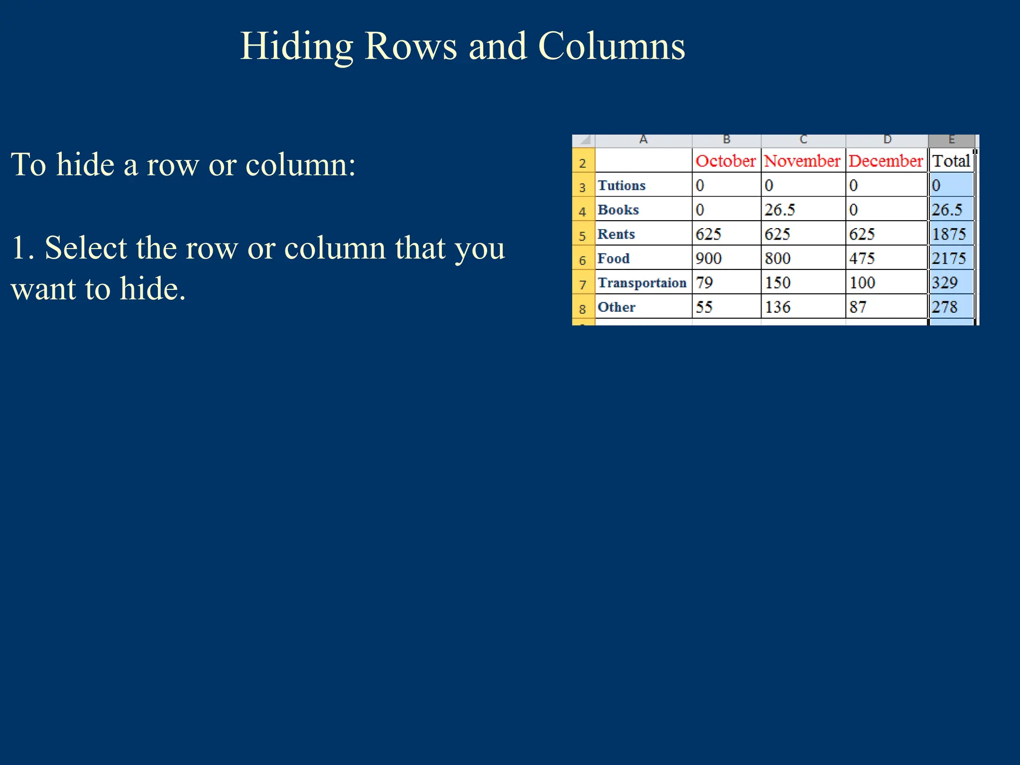
45. Hiding Rows and Columns
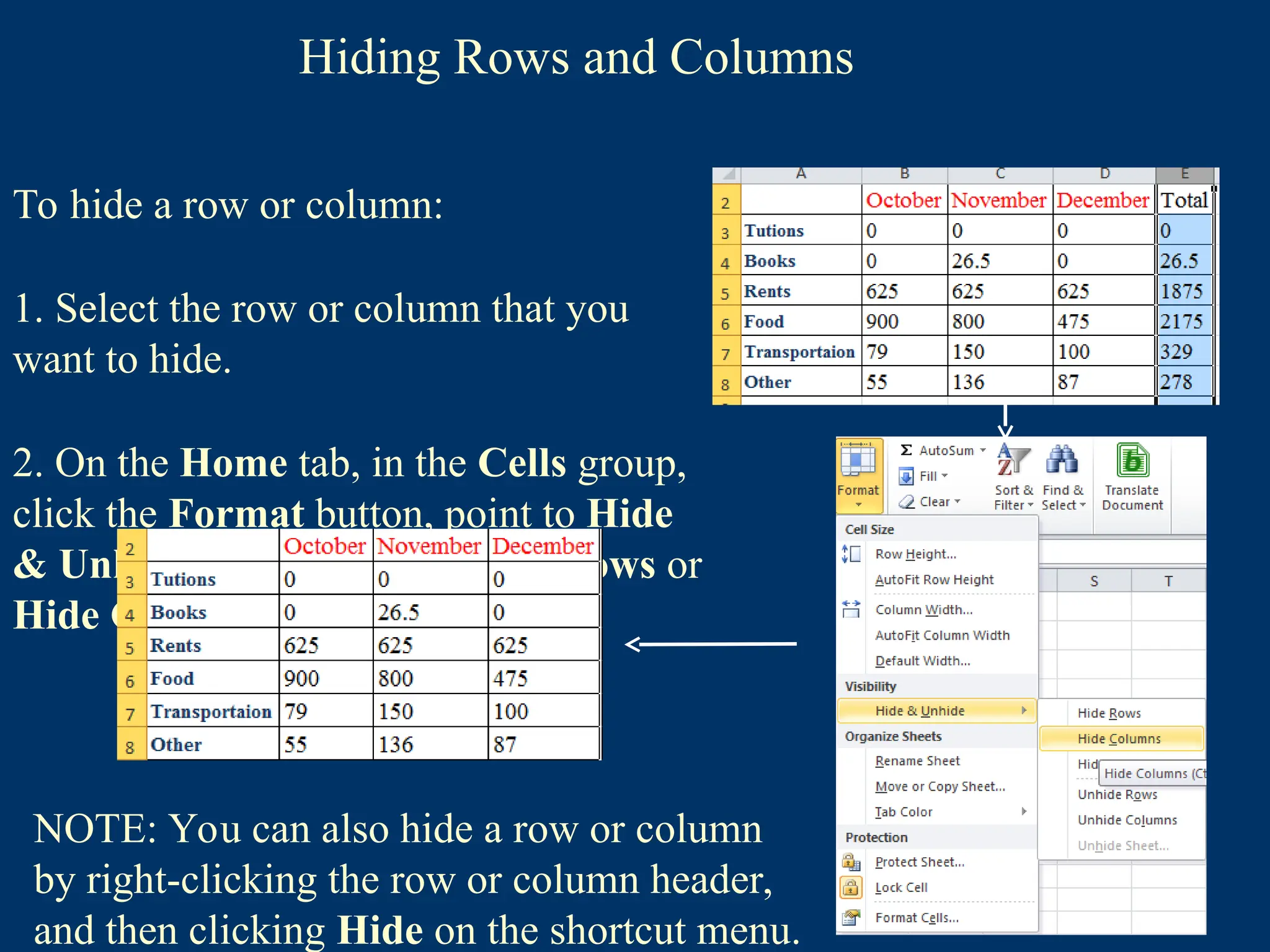
To hide a row or column:
1. Select the row or column that you
want to hide.

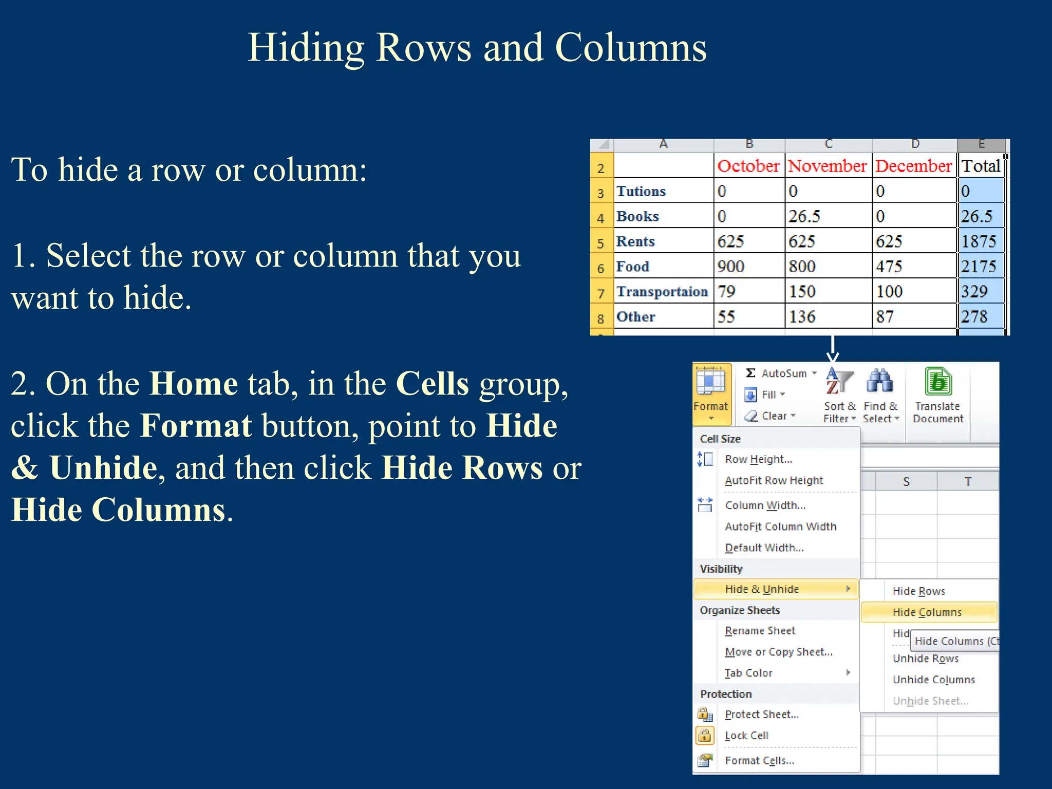
46. Hiding Rows and Columns
To hide a row or column:
1. Select the row or column that you
want to hide.
2. On the Home tab, in the Cells group,
click the Format button, point to Hide
& Unhide, and then click Hide Rows or
Hide Columns.

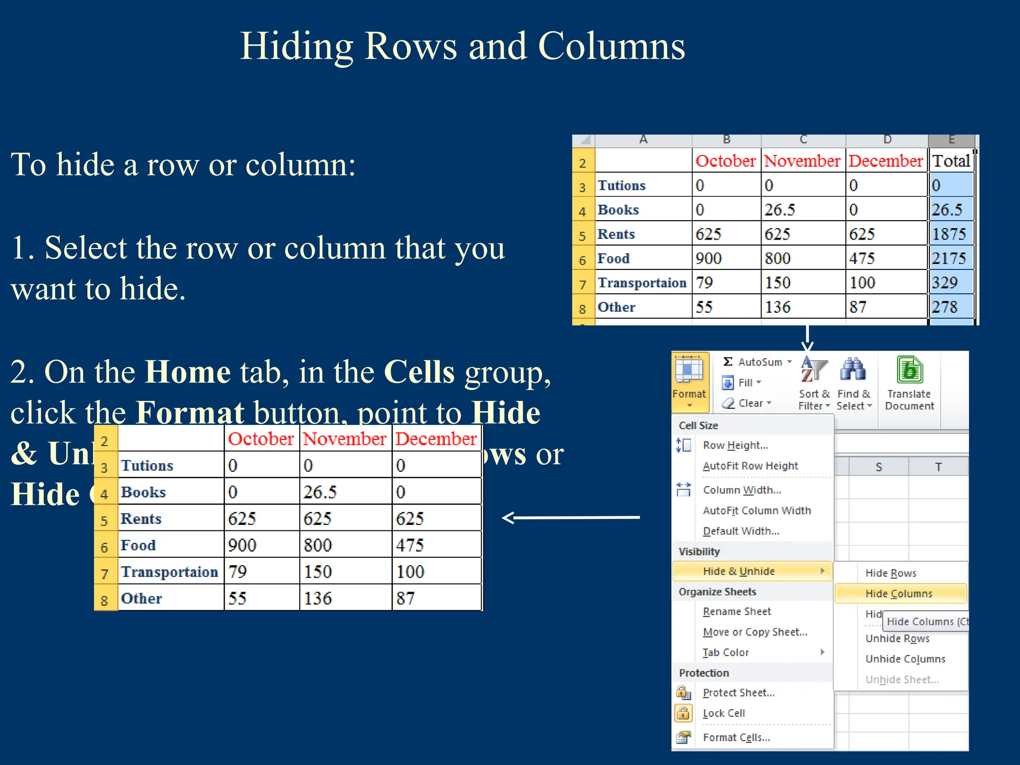
47. Hiding Rows and Columns
To hide a row or column:
1. Select the row or column that you
want to hide.
2. On the Home tab, in the Cells group,
click the Format button, point to Hide
& Unhide, and then click Hide Rows or
Hide Columns.

48. Hiding Rows and Columns
To hide a row or column:
1. Select the row or column that you
want to hide.
2. On the Home tab, in the Cells group,
click the Format button, point to Hide
& Unhide, and then click Hide Rows or
Hide Columns.
NOTE: You can also hide a row or column
by right-clicking the row or column header,
and then clicking Hide on the shortcut menu.

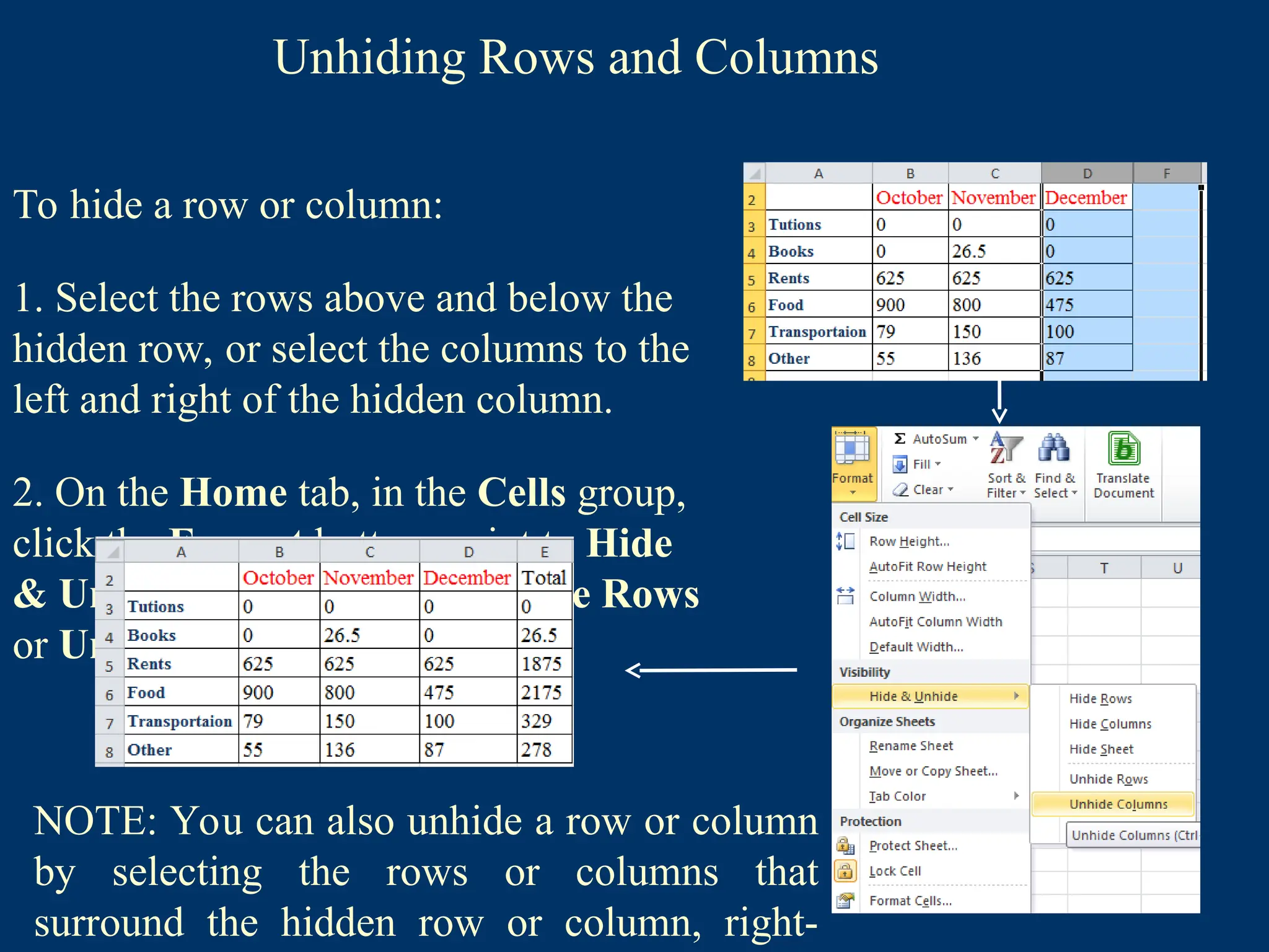
49. Unhiding Rows and Columns
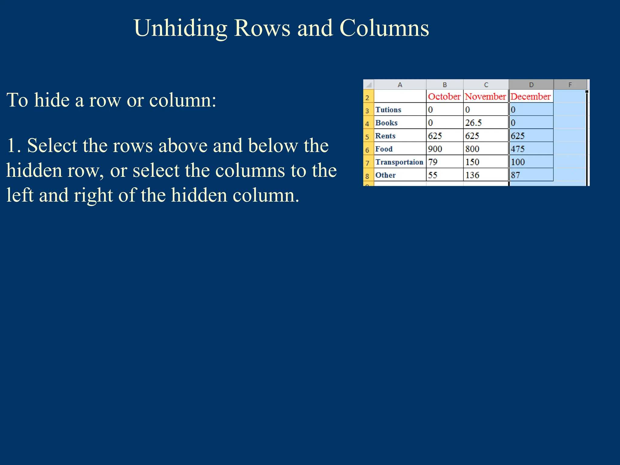
To hide a row or column:
1. Select the rows above and below the
hidden row, or select the columns to the
left and right of the hidden column.

50. Unhiding Rows and Columns
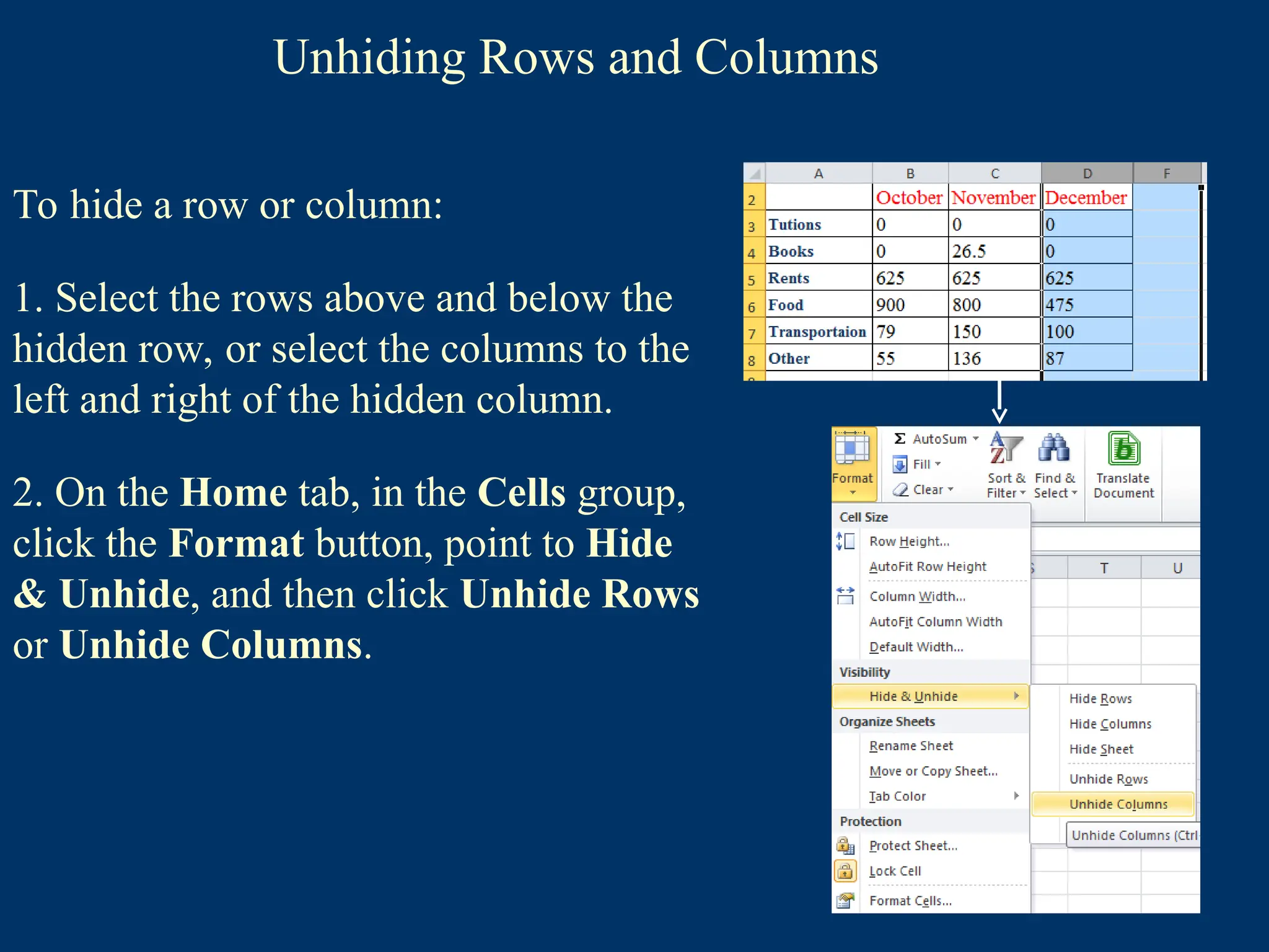
To hide a row or column:
1. Select the rows above and below the
hidden row, or select the columns to the
left and right of the hidden column.
2. On the Home tab, in the Cells group,
click the Format button, point to Hide
& Unhide, and then click Unhide Rows
or Unhide Columns.

51. Unhiding Rows and Columns
To hide a row or column:
1. Select the rows above and below the
hidden row, or select the columns to the
left and right of the hidden column.
2. On the Home tab, in the Cells group,
click the Format button, point to Hide
& Unhide, and then click Unhide Rows
or Unhide Columns.

52. Unhiding Rows and Columns
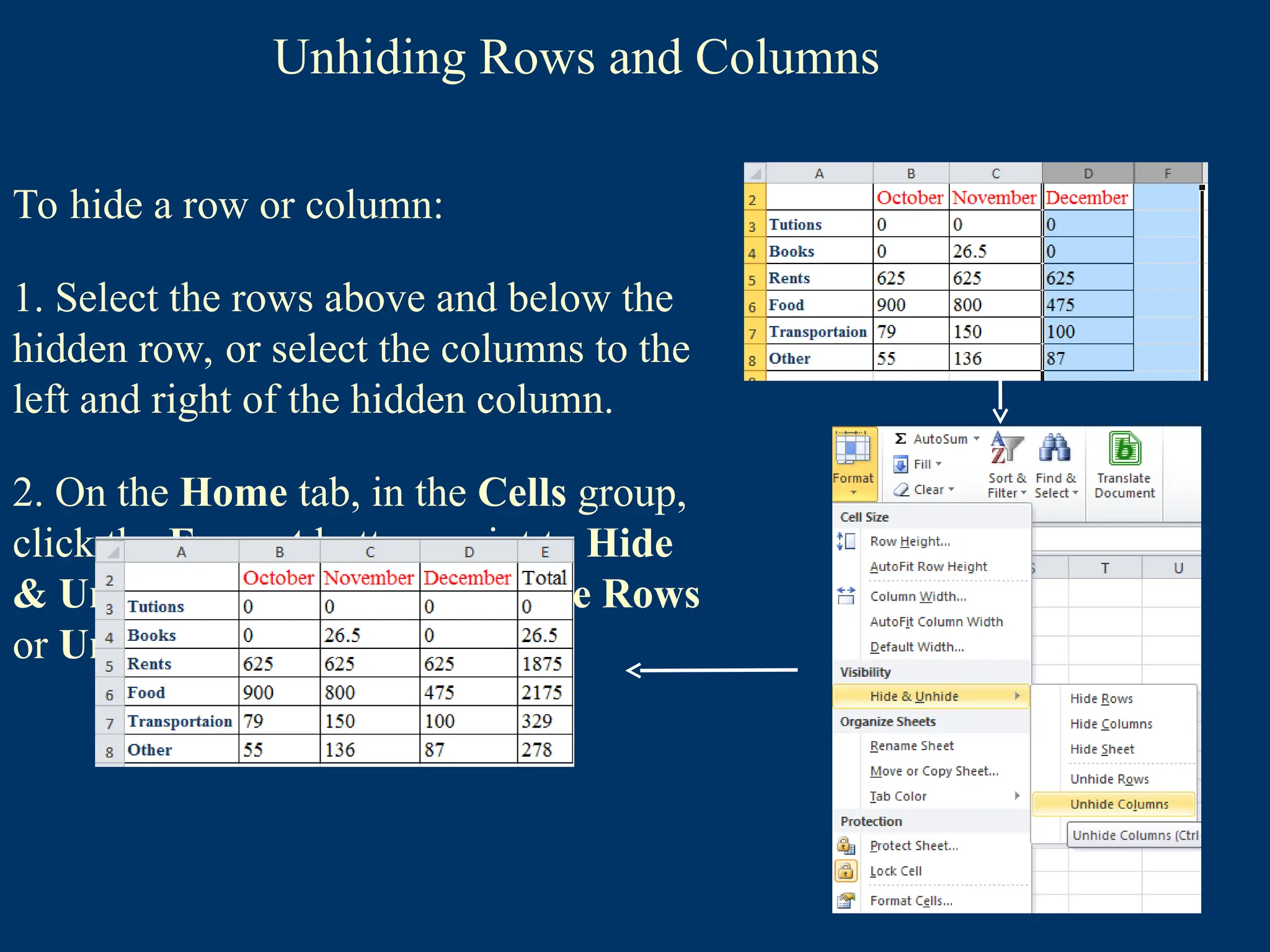
To hide a row or column:
1. Select the rows above and below the
hidden row, or select the columns to the
left and right of the hidden column.
2. On the Home tab, in the Cells group,
click the Format button, point to Hide
& Unhide, and then click Unhide Rows
or Unhide Columns.
NOTE: You can also unhide a row or column
by selecting the rows or columns that
surround the hidden row or column, right-

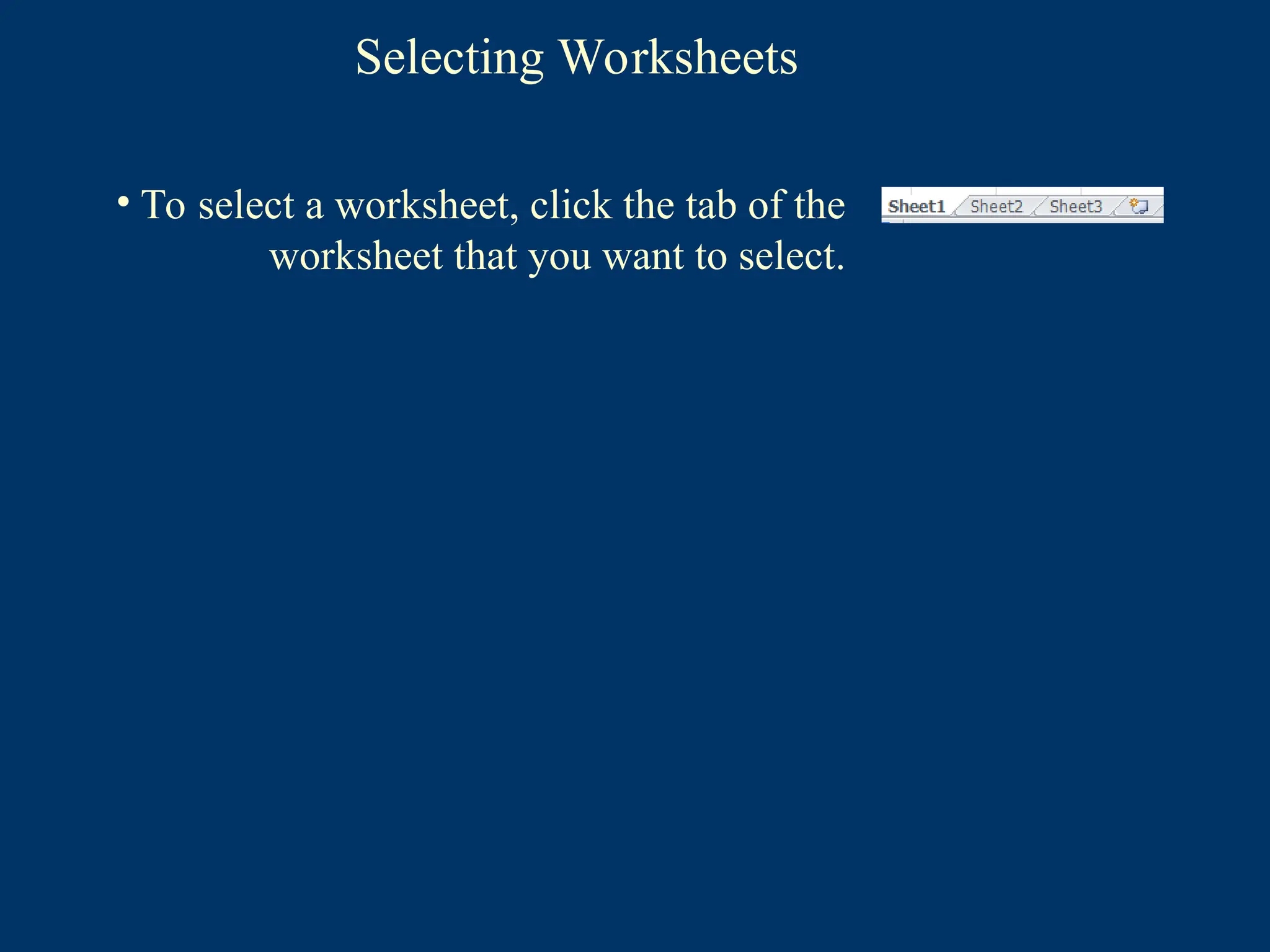
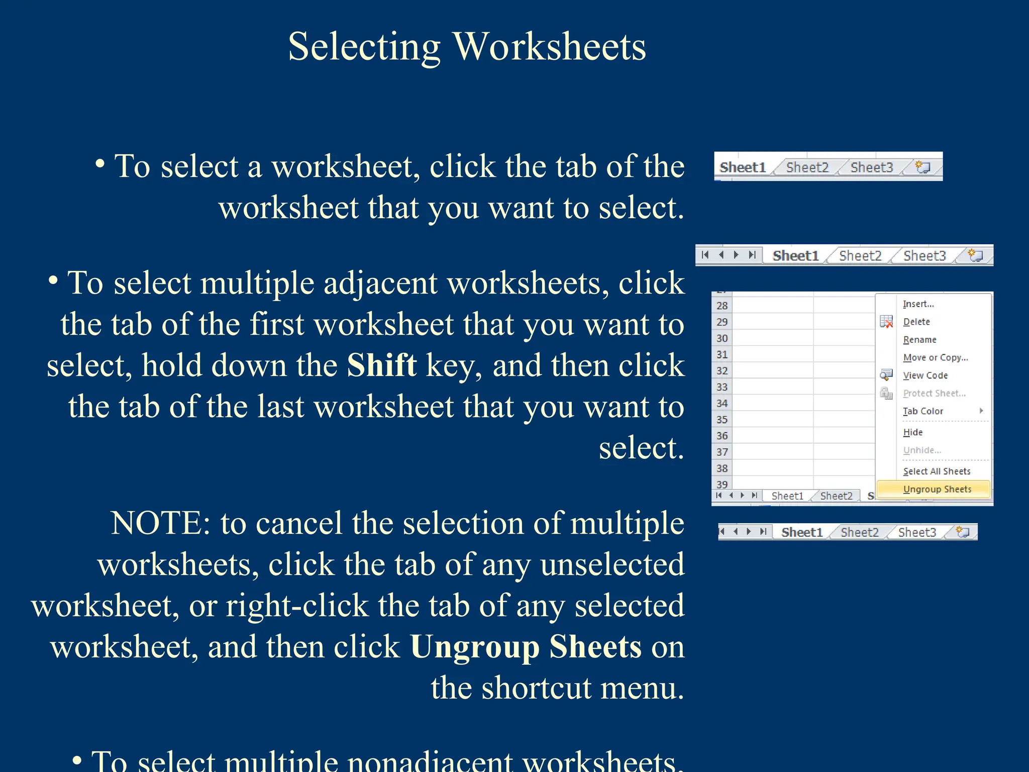
53. Selecting Worksheets
• To select a worksheet, click the tab of the
worksheet that you want to select.

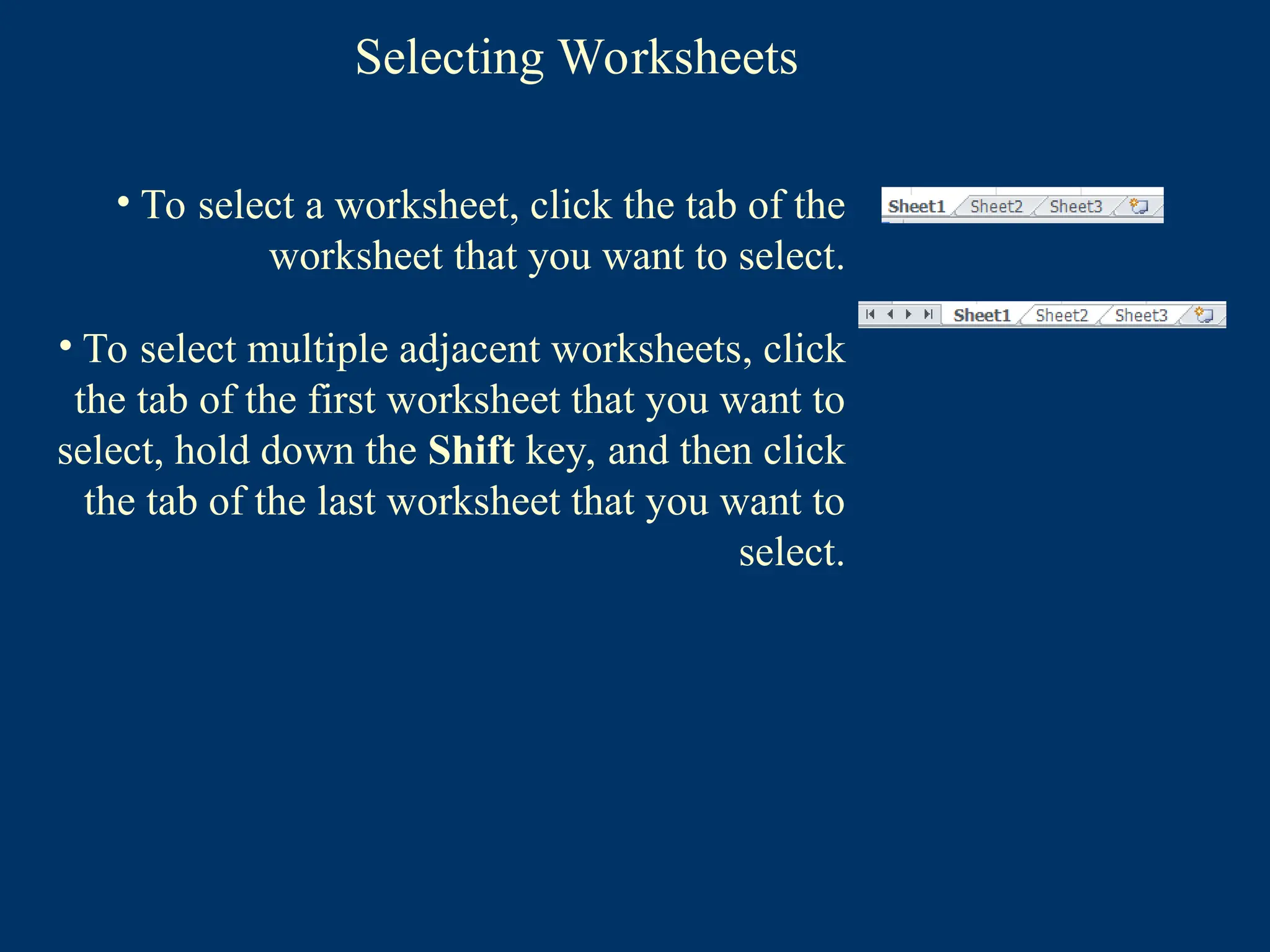
54. Selecting Worksheets
• To select a worksheet, click the tab of the
worksheet that you want to select.
• To select multiple adjacent worksheets, click
the tab of the first worksheet that you want to
select, hold down the Shift key, and then click
the tab of the last worksheet that you want to
select.

55. Selecting Worksheets
• To select a worksheet, click the tab of the
worksheet that you want to select.
• To select multiple adjacent worksheets, click
the tab of the first worksheet that you want to
select, hold down the Shift key, and then click
the tab of the last worksheet that you want to
select.
NOTE: to cancel the selection of multiple
worksheets, click the tab of any unselected
worksheet, or right-click the tab of any selected
worksheet, and then click Ungroup Sheets on
the shortcut menu.

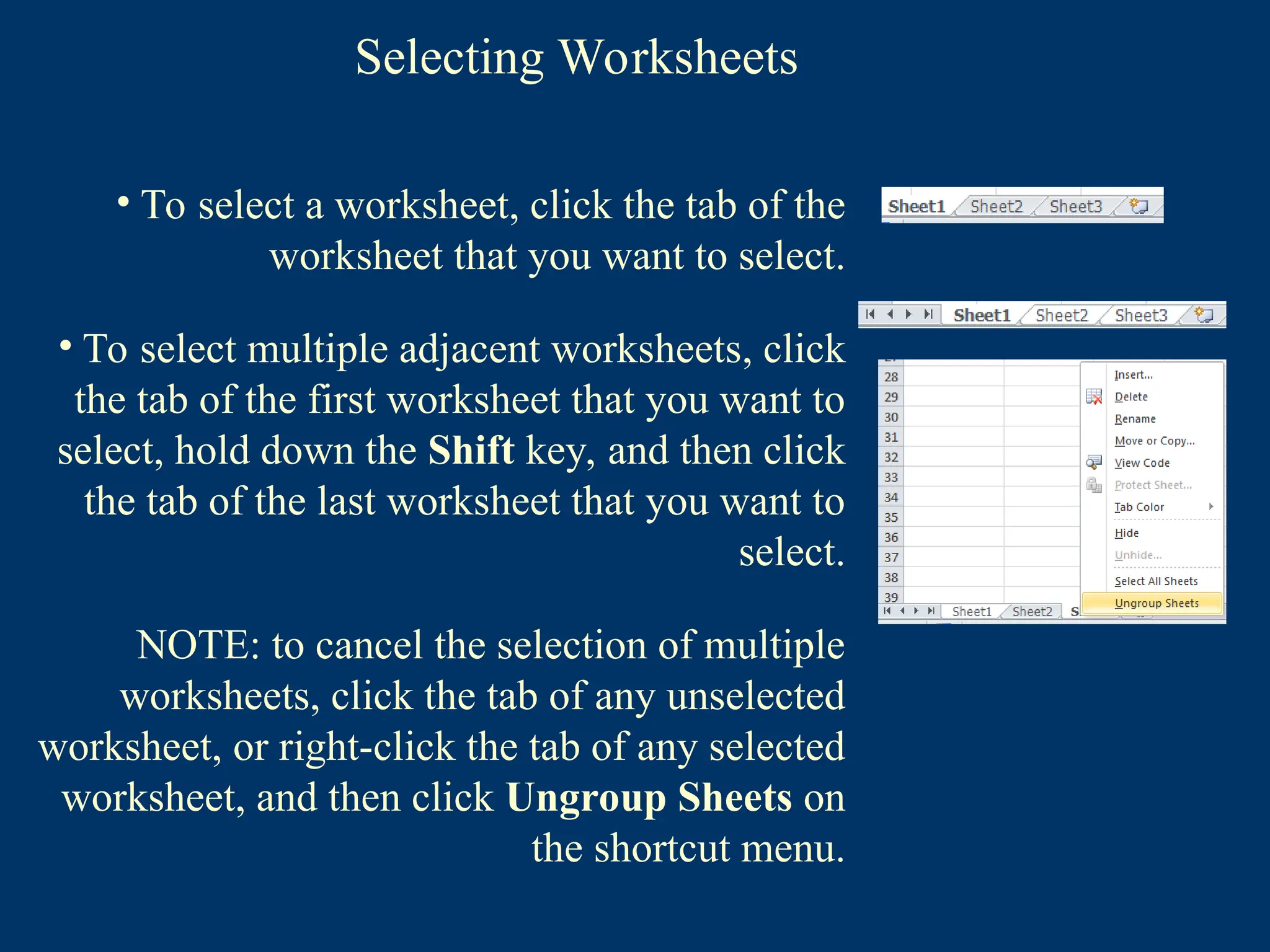
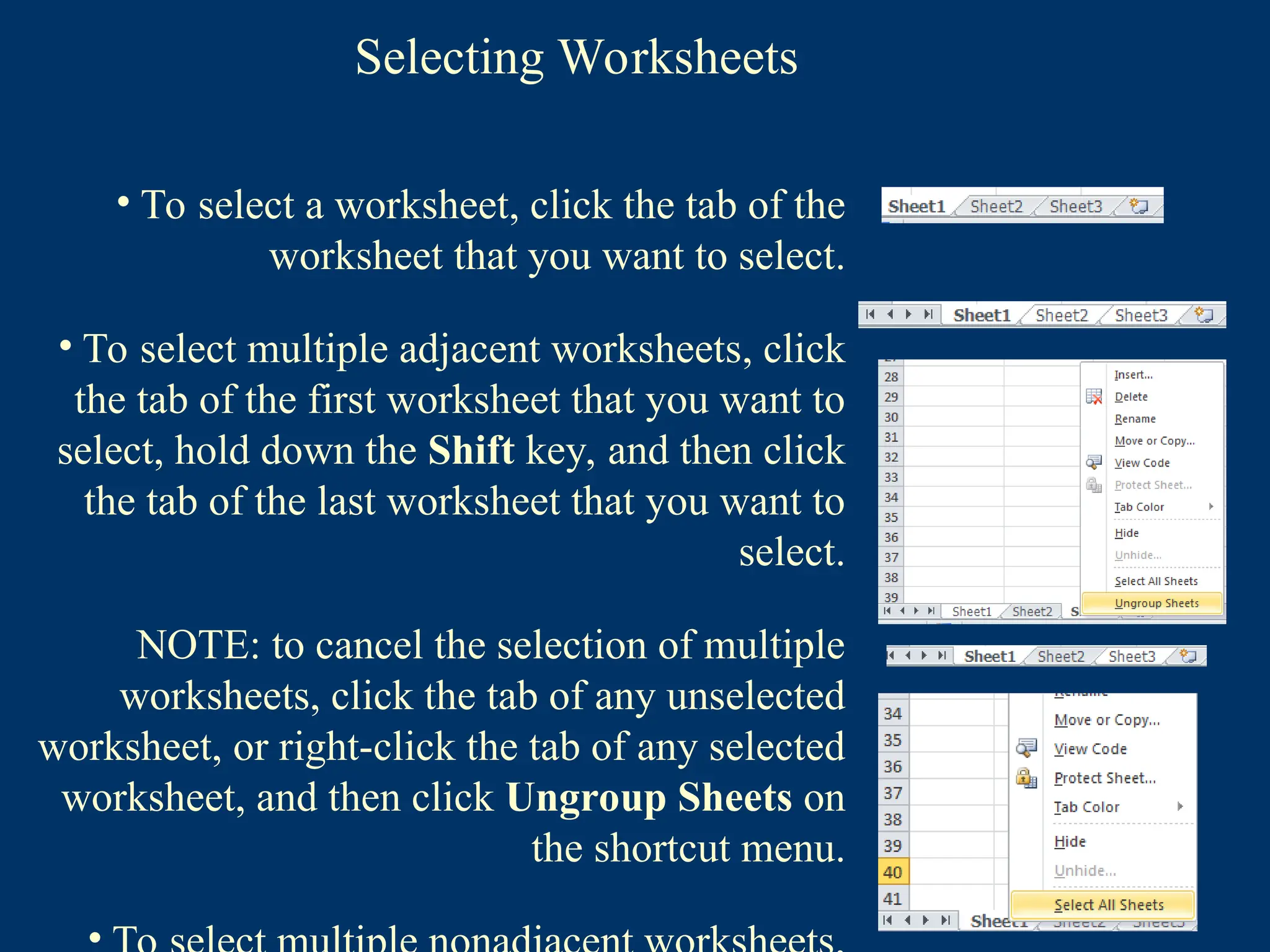
56. Selecting Worksheets
• To select a worksheet, click the tab of the
worksheet that you want to select.
• To select multiple adjacent worksheets, click
the tab of the first worksheet that you want to
select, hold down the Shift key, and then click
the tab of the last worksheet that you want to
select.
NOTE: to cancel the selection of multiple
worksheets, click the tab of any unselected
worksheet, or right-click the tab of any selected
worksheet, and then click Ungroup Sheets on
the shortcut menu.

57. Selecting Worksheets
• To select a worksheet, click the tab of the
worksheet that you want to select.
• To select multiple adjacent worksheets, click
the tab of the first worksheet that you want to
select, hold down the Shift key, and then click
the tab of the last worksheet that you want to
select.
NOTE: to cancel the selection of multiple
worksheets, click the tab of any unselected
worksheet, or right-click the tab of any selected
worksheet, and then click Ungroup Sheets on
the shortcut menu.

58. Navigating Between Worksheets
If a workbook contains many worksheets, all the worksheet tabs
may not be visible.

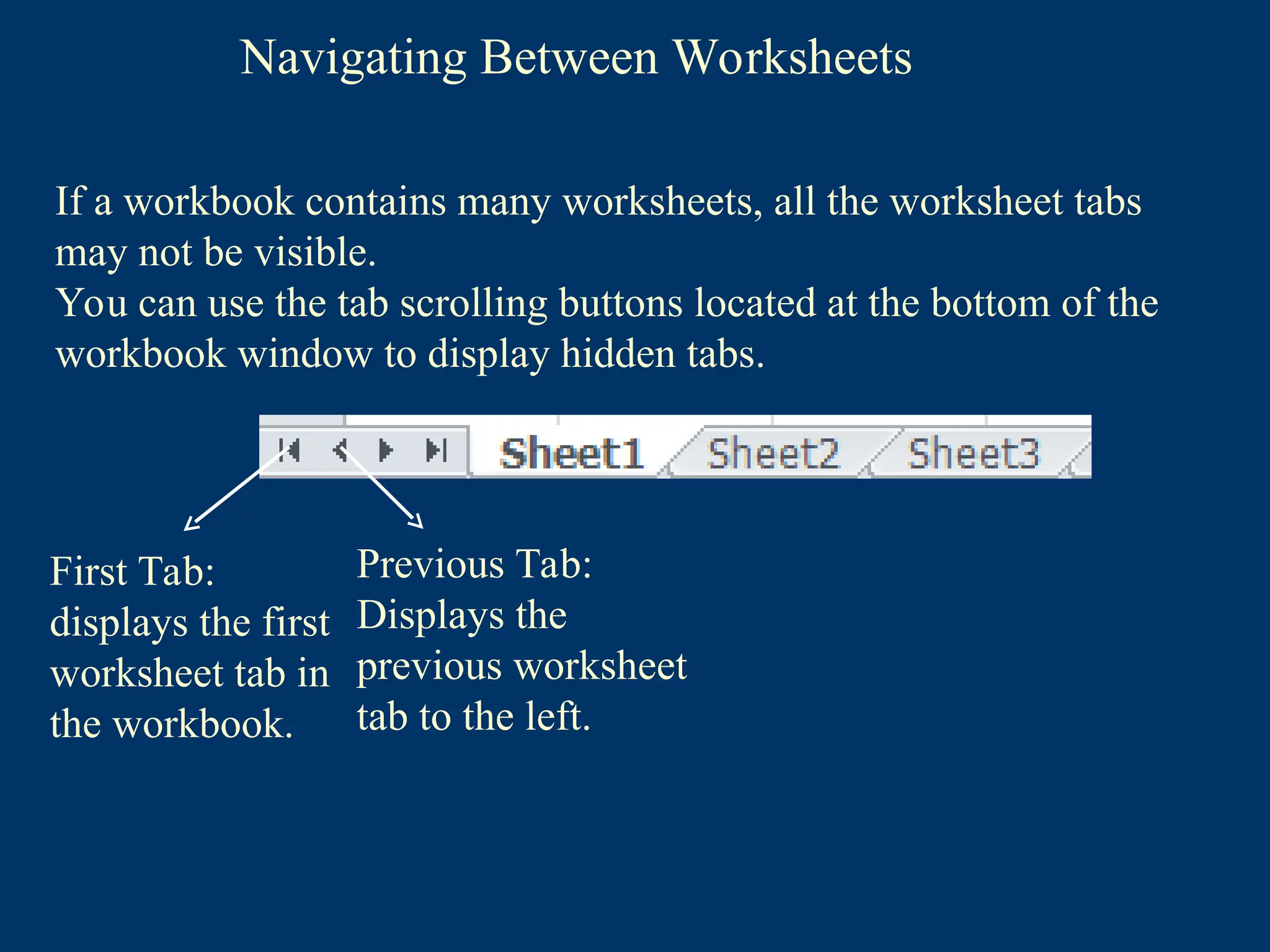
59. Navigating Between Worksheets
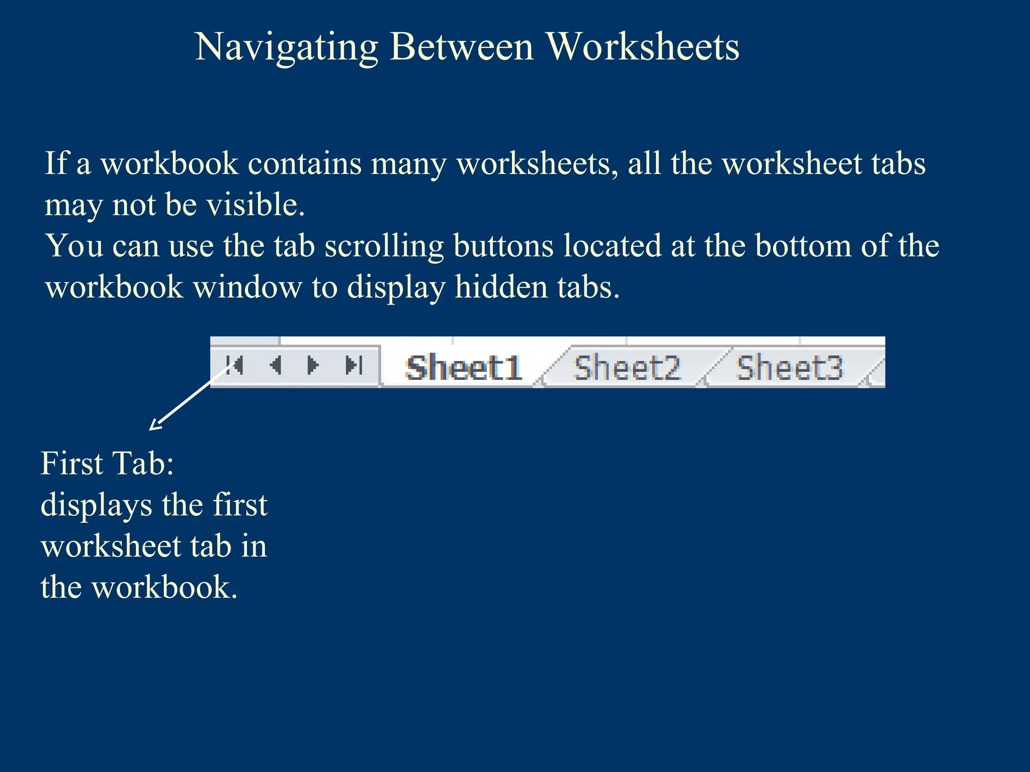
If a workbook contains many worksheets, all the worksheet tabs
may not be visible.
You can use the tab scrolling buttons located at the bottom of the
workbook window to display hidden tabs.

60. Navigating Between Worksheets
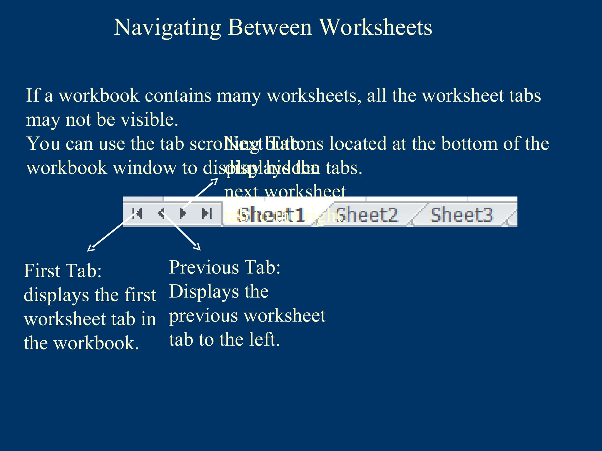
First Tab:
displays the first
worksheet tab in
the workbook.
If a workbook contains many worksheets, all the worksheet tabs
may not be visible.
You can use the tab scrolling buttons located at the bottom of the
workbook window to display hidden tabs.

61. Navigating Between Worksheets
First Tab:
displays the first
worksheet tab in
the workbook.
Previous Tab:
Displays the
previous worksheet
tab to the left.
If a workbook contains many worksheets, all the worksheet tabs
may not be visible.
You can use the tab scrolling buttons located at the bottom of the
workbook window to display hidden tabs.

62. Navigating Between Worksheets
First Tab:
displays the first
worksheet tab in
the workbook.
Previous Tab:
Displays the
previous worksheet
tab to the left.
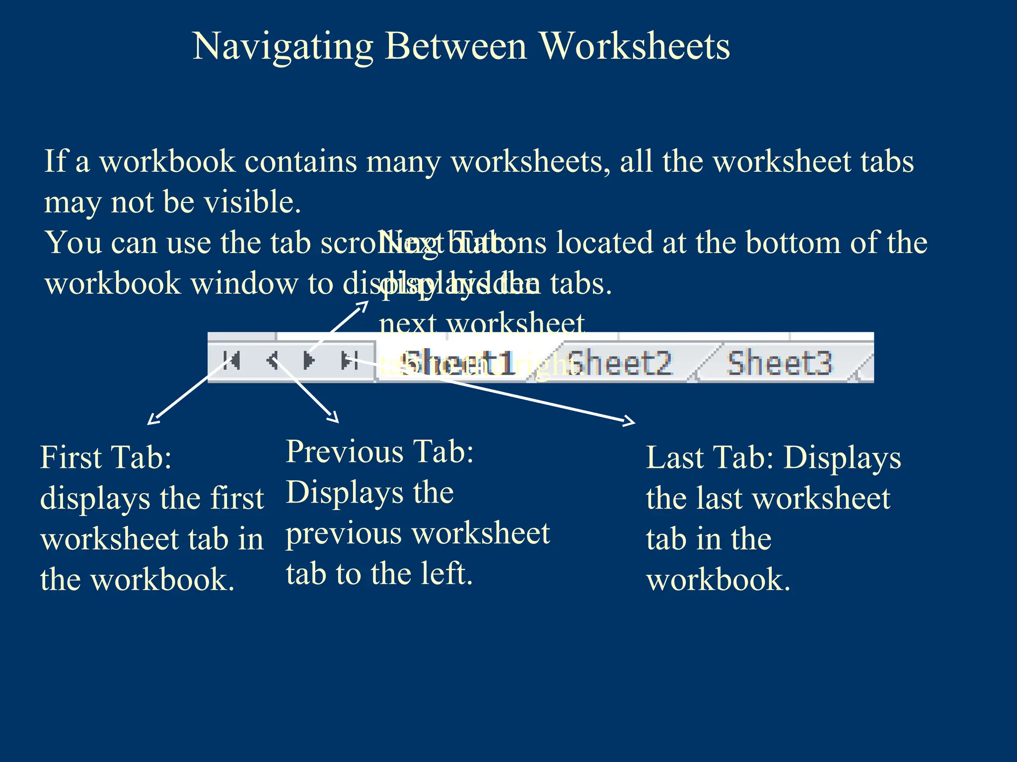
Next Tab:
displays the
next worksheet
tab to the right.
If a workbook contains many worksheets, all the worksheet tabs
may not be visible.
You can use the tab scrolling buttons located at the bottom of the
workbook window to display hidden tabs.

63. Navigating Between Worksheets
First Tab:
displays the first
worksheet tab in
the workbook.
Previous Tab:
Displays the
previous worksheet
tab to the left.
Next Tab:
displays the
next worksheet
tab to the right.
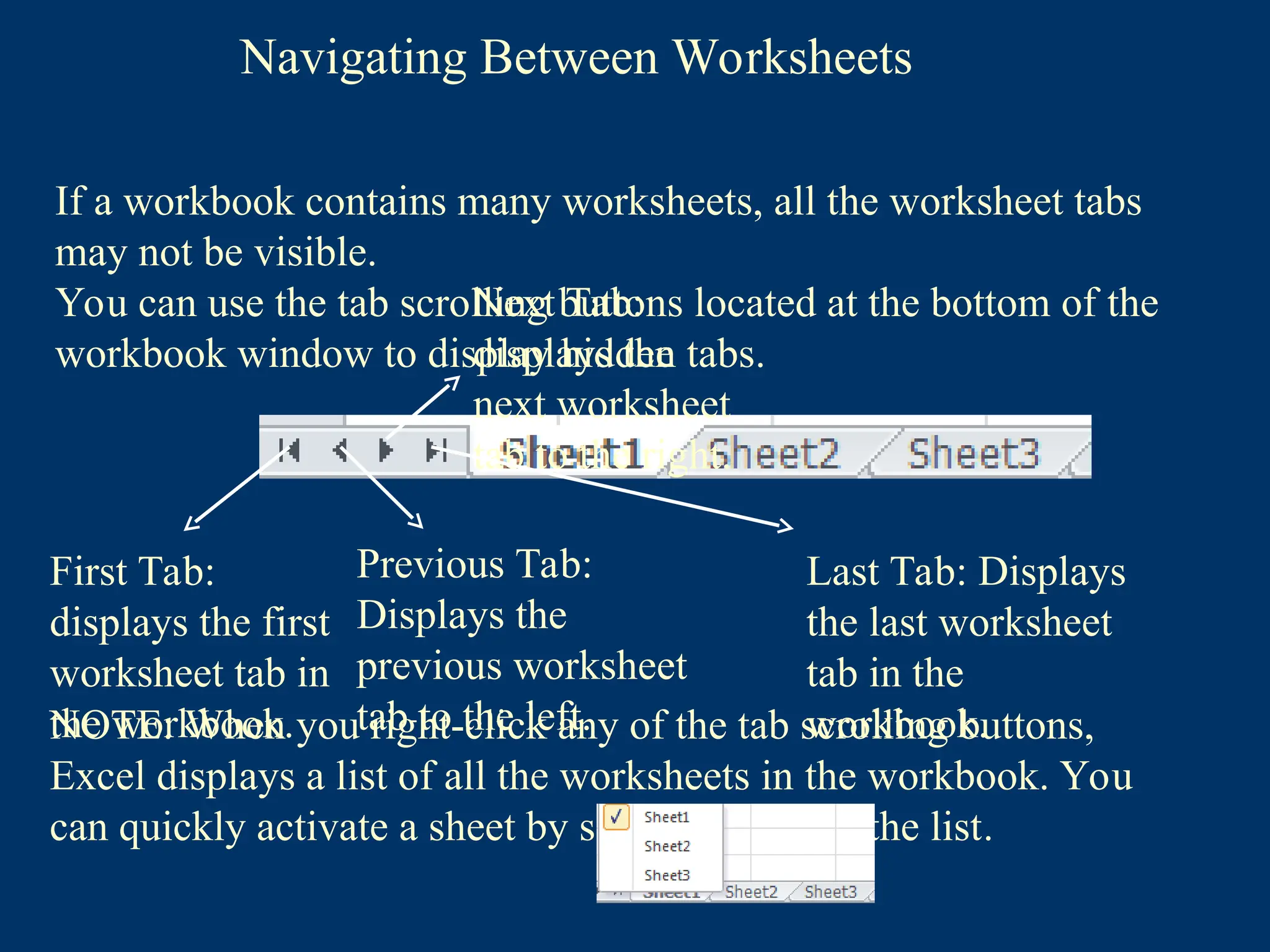
Last Tab: Displays
the last worksheet
tab in the
workbook.
If a workbook contains many worksheets, all the worksheet tabs
may not be visible.
You can use the tab scrolling buttons located at the bottom of the
workbook window to display hidden tabs.

64. Navigating Between Worksheets
First Tab:
displays the first
worksheet tab in
the workbook.
Previous Tab:
Displays the
previous worksheet
tab to the left.
Next Tab:
displays the
next worksheet
tab to the right.
Last Tab: Displays
the last worksheet
tab in the
workbook.
If a workbook contains many worksheets, all the worksheet tabs
may not be visible.
You can use the tab scrolling buttons located at the bottom of the
workbook window to display hidden tabs.
NOTE: When you right-click any of the tab scrolling buttons,
Excel displays a list of all the worksheets in the workbook. You
can quickly activate a sheet by selecting it from the list.

65. Renaming Worksheets
To rename a worksheet:
•Double-click the tab of the worksheet that you want to rename.
Or, right-click the worksheet tab, and then click Rename on the
shortcut menu

66. Renaming Worksheets
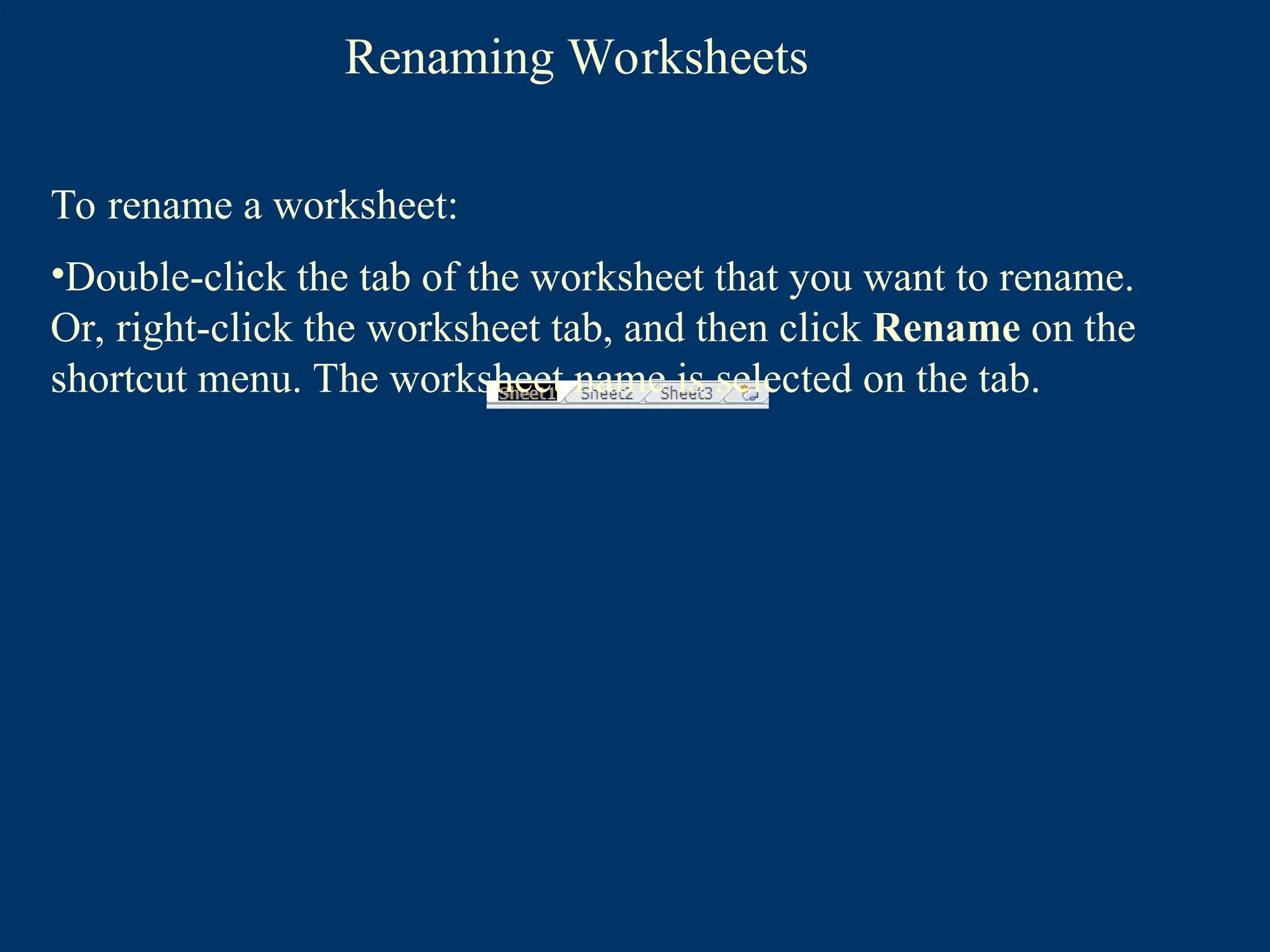
To rename a worksheet:
•Double-click the tab of the worksheet that you want to rename.
Or, right-click the worksheet tab, and then click Rename on the
shortcut menu. The worksheet name is selected on the tab.

67. Renaming Worksheets
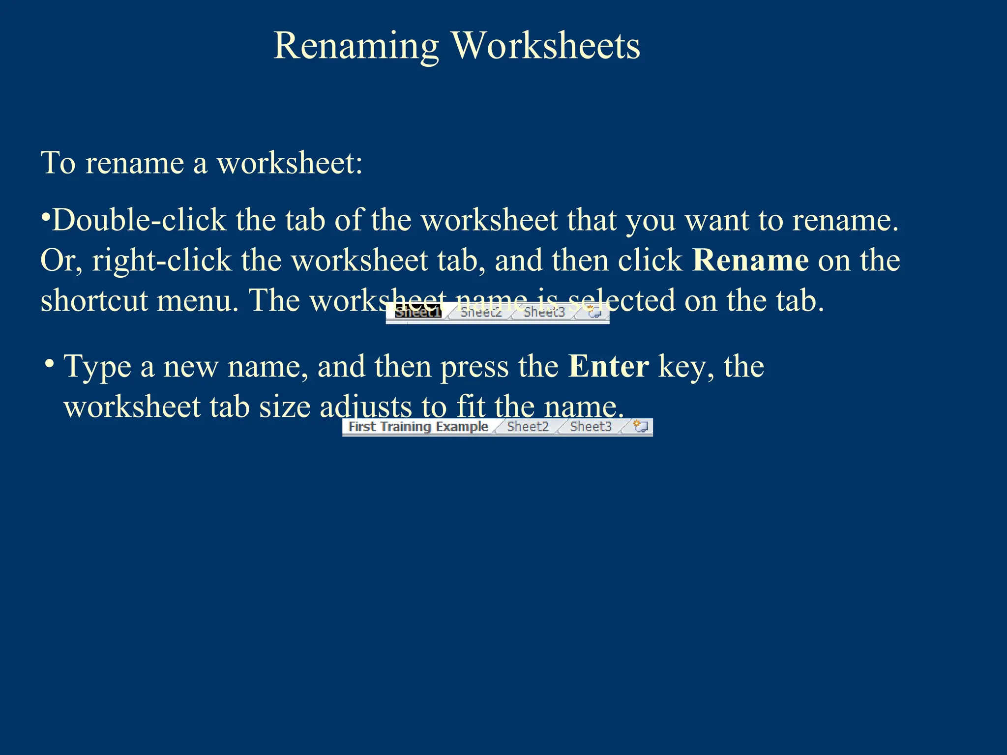
• Type a new name, and then press the Enter key, the
worksheet tab size adjusts to fit the name.
To rename a worksheet:
•Double-click the tab of the worksheet that you want to rename.
Or, right-click the worksheet tab, and then click Rename on the
shortcut menu. The worksheet name is selected on the tab.

68. Renaming Worksheets
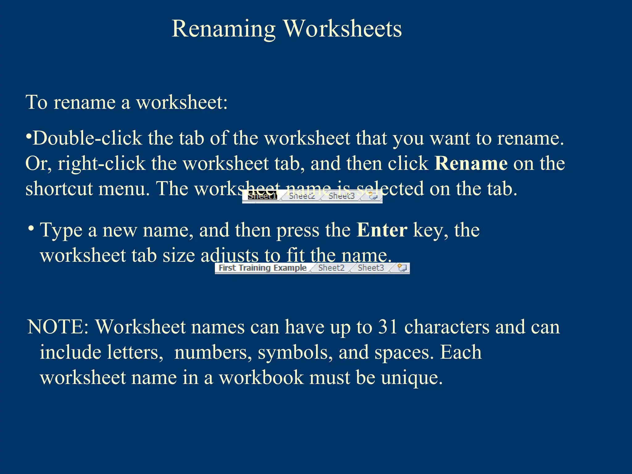
• Type a new name, and then press the Enter key, the
worksheet tab size adjusts to fit the name.
NOTE: Worksheet names can have up to 31 characters and can
include letters, numbers, symbols, and spaces. Each
worksheet name in a workbook must be unique.
To rename a worksheet:
•Double-click the tab of the worksheet that you want to rename.
Or, right-click the worksheet tab, and then click Rename on the
shortcut menu. The worksheet name is selected on the tab.

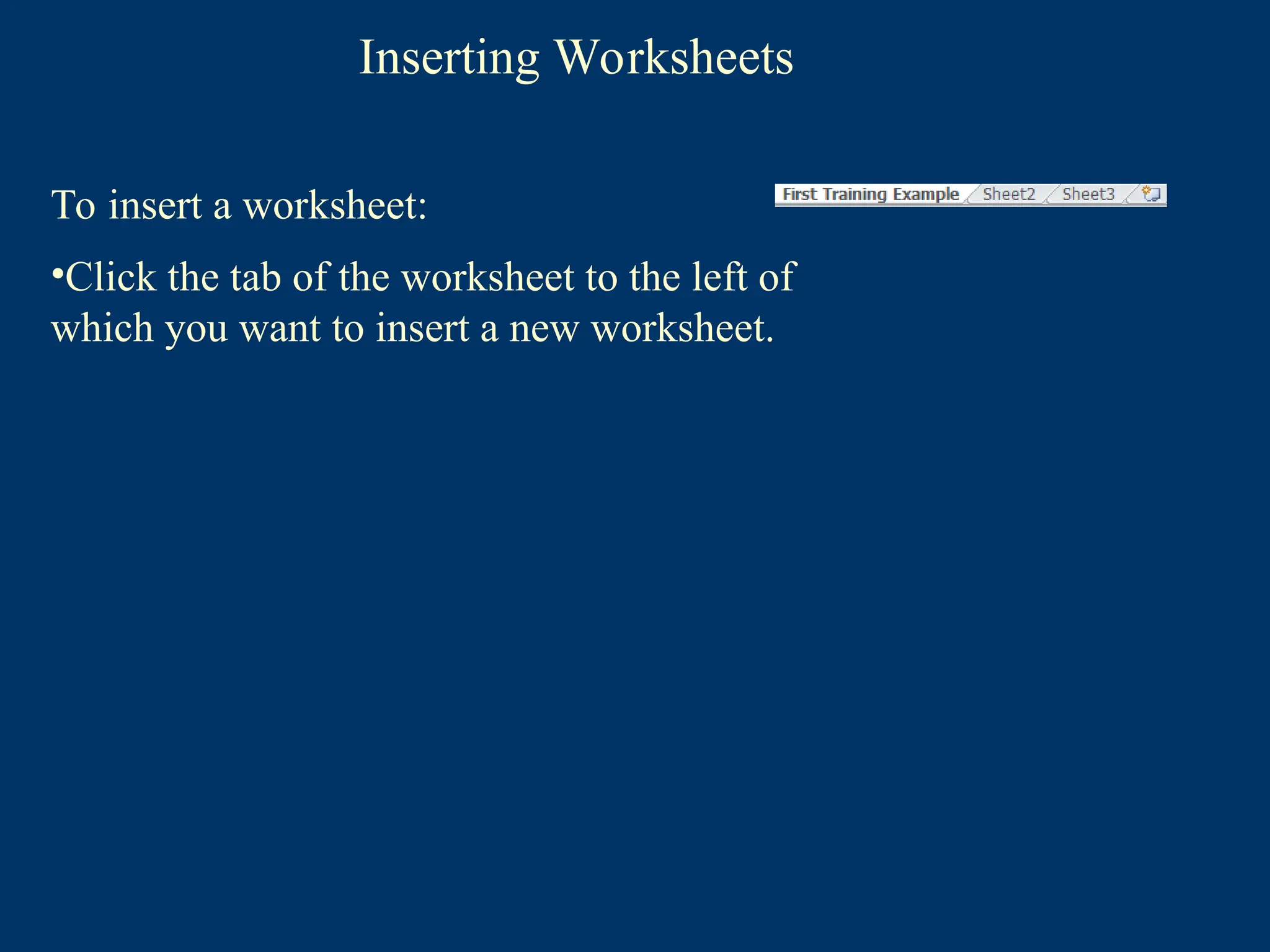
69. Inserting Worksheets
To insert a worksheet:
•Click the tab of the worksheet to the left of
which you want to insert a new worksheet.

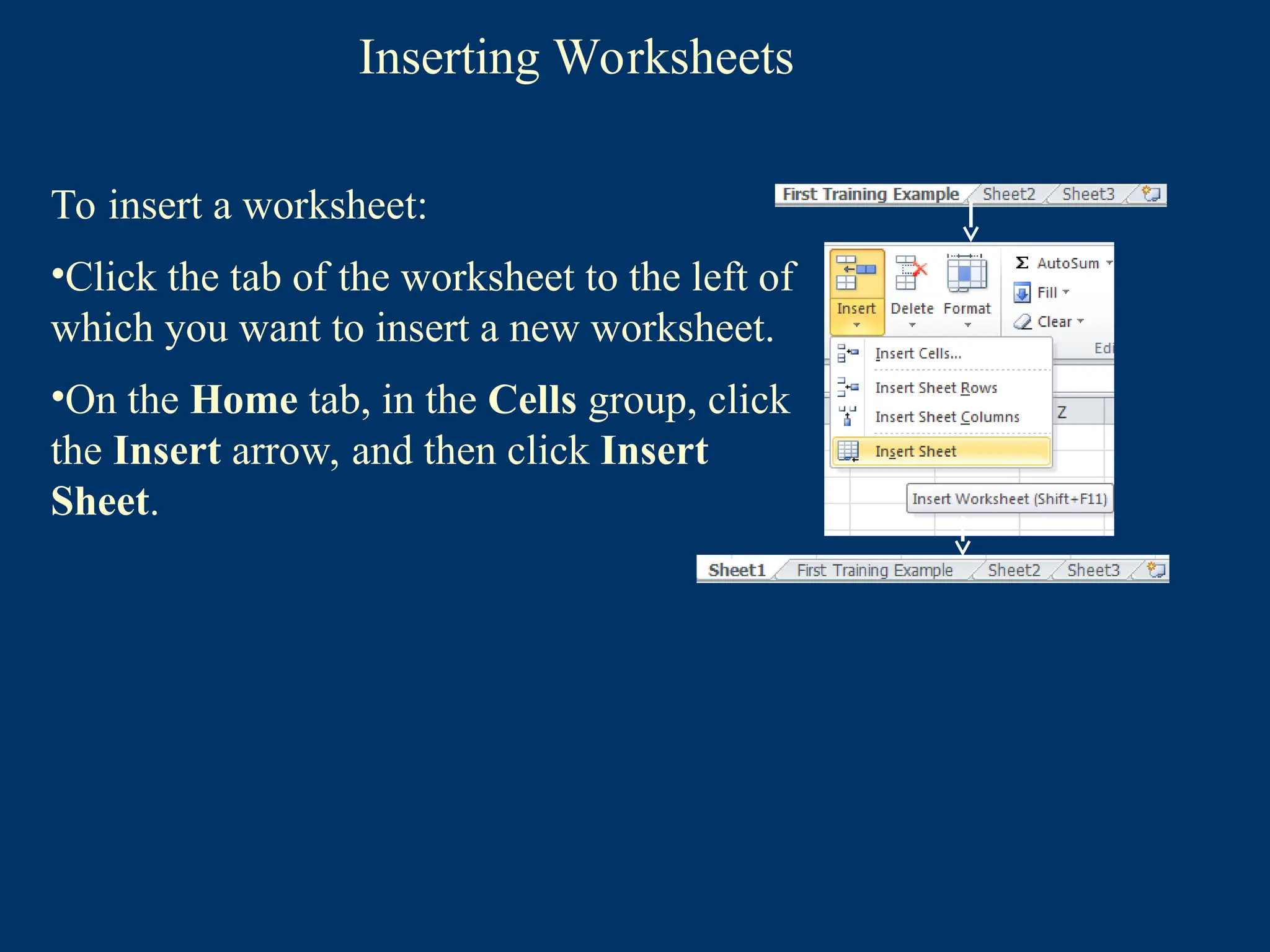
70. Inserting Worksheets
To insert a worksheet:
•Click the tab of the worksheet to the left of
which you want to insert a new worksheet.
•On the Home tab, in the Cells group, click
the Insert arrow, and then click Insert
Sheet.

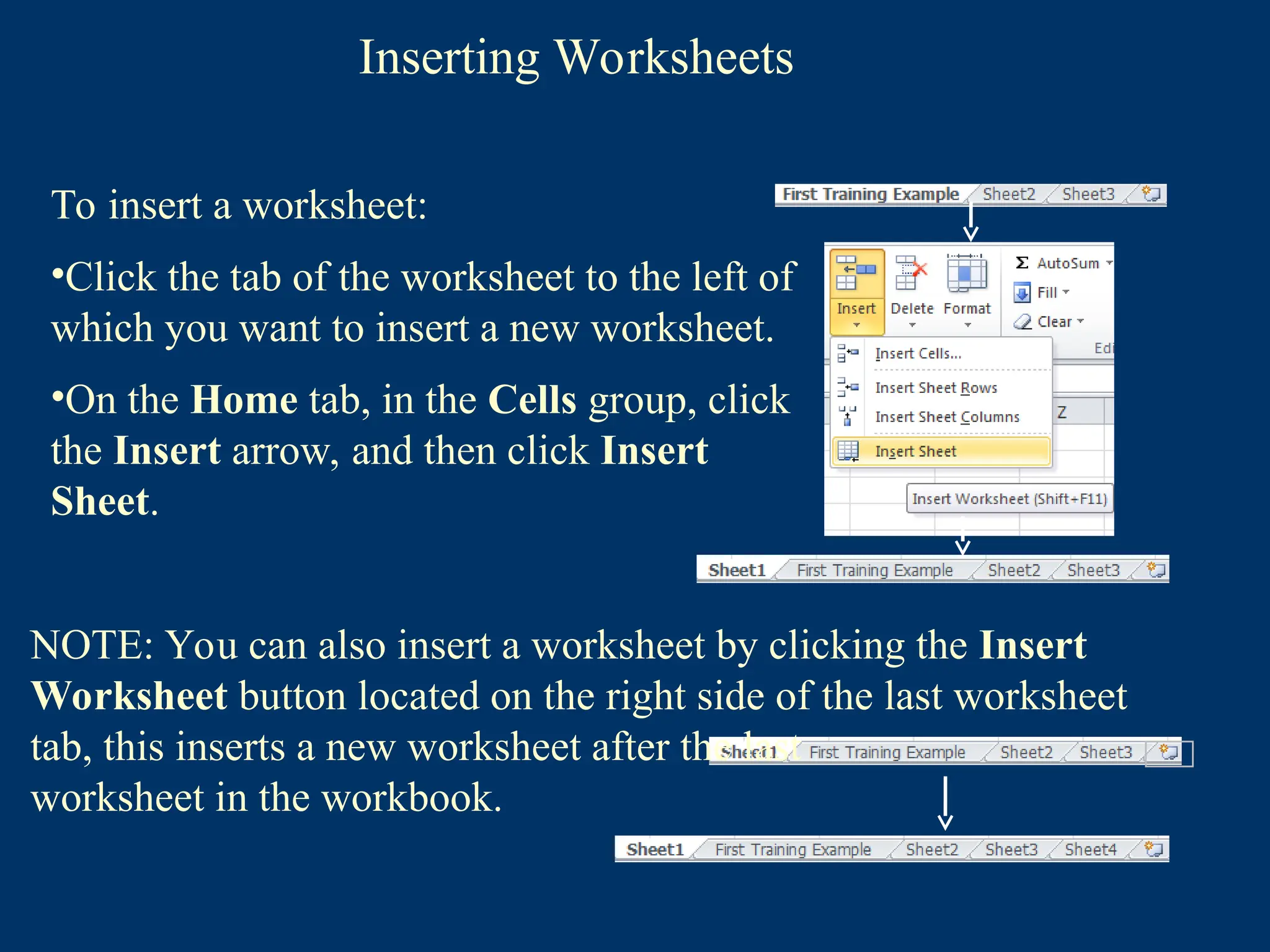
71. Inserting Worksheets
To insert a worksheet:
•Click the tab of the worksheet to the left of
which you want to insert a new worksheet.
•On the Home tab, in the Cells group, click
the Insert arrow, and then click Insert
Sheet.
NOTE: You can also insert a worksheet by clicking the Insert
Worksheet button located on the right side of the last worksheet
tab, this inserts a new worksheet after the last
worksheet in the workbook.

72. Deleting Worksheets
To delete a worksheet:
•Click the tab of the worksheet that you want to
delete.

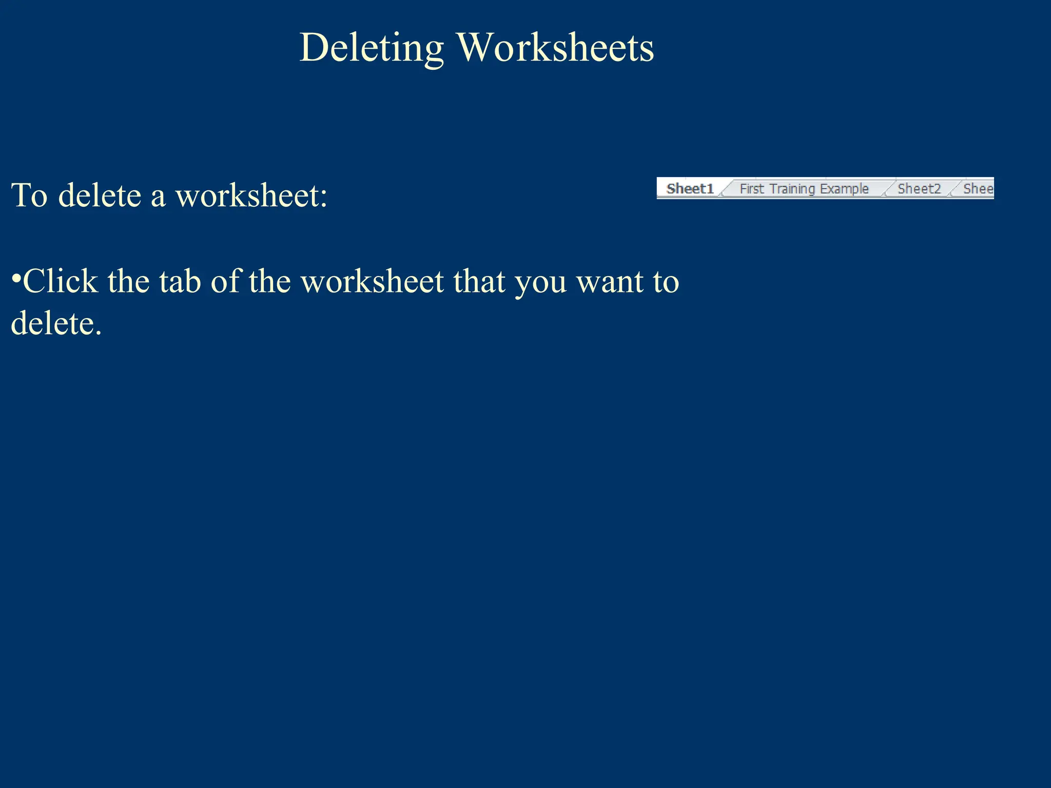
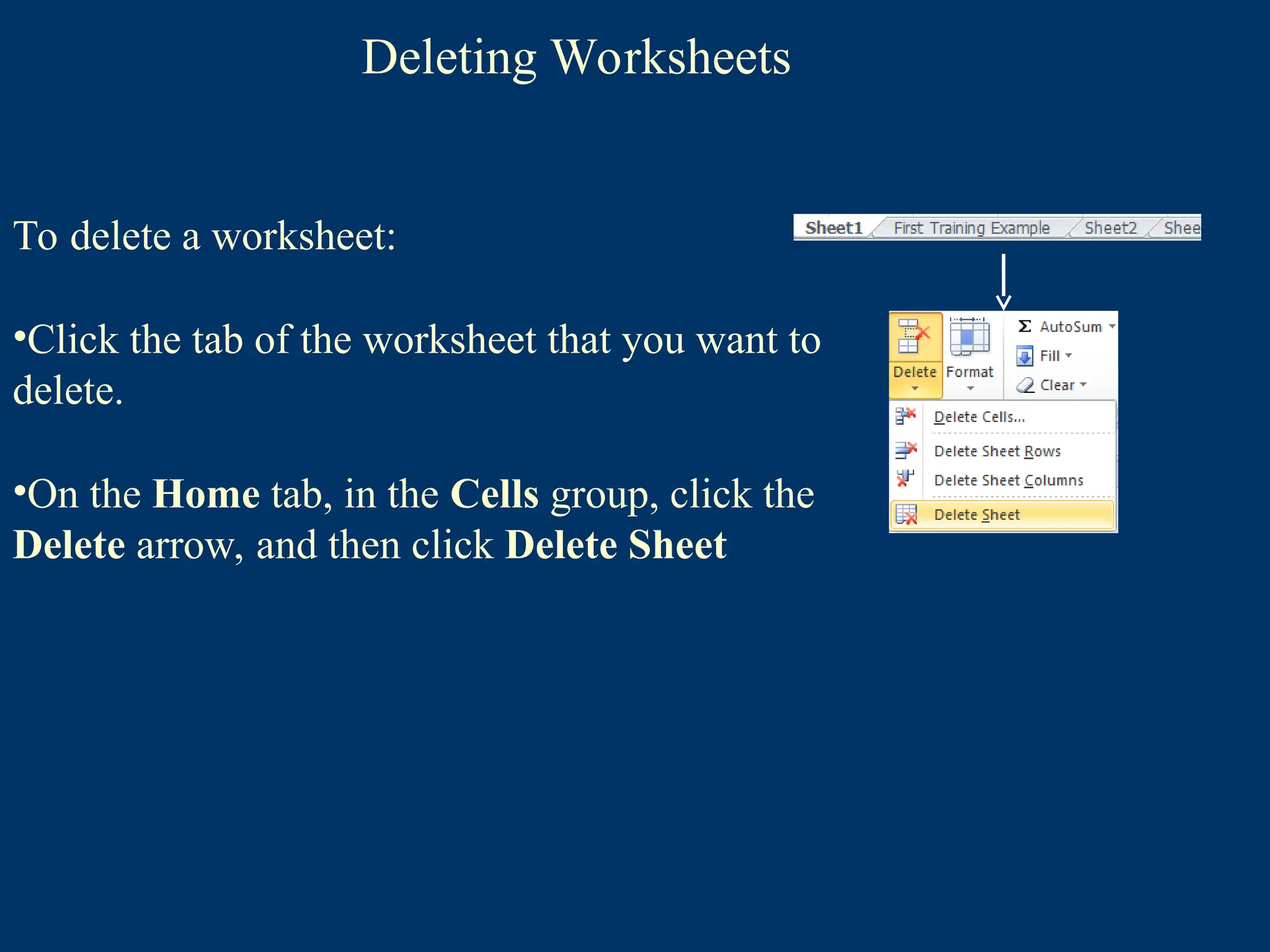
73. Deleting Worksheets
To delete a worksheet:
•Click the tab of the worksheet that you want to
delete.
•On the Home tab, in the Cells group, click the
Delete arrow, and then click Delete Sheet

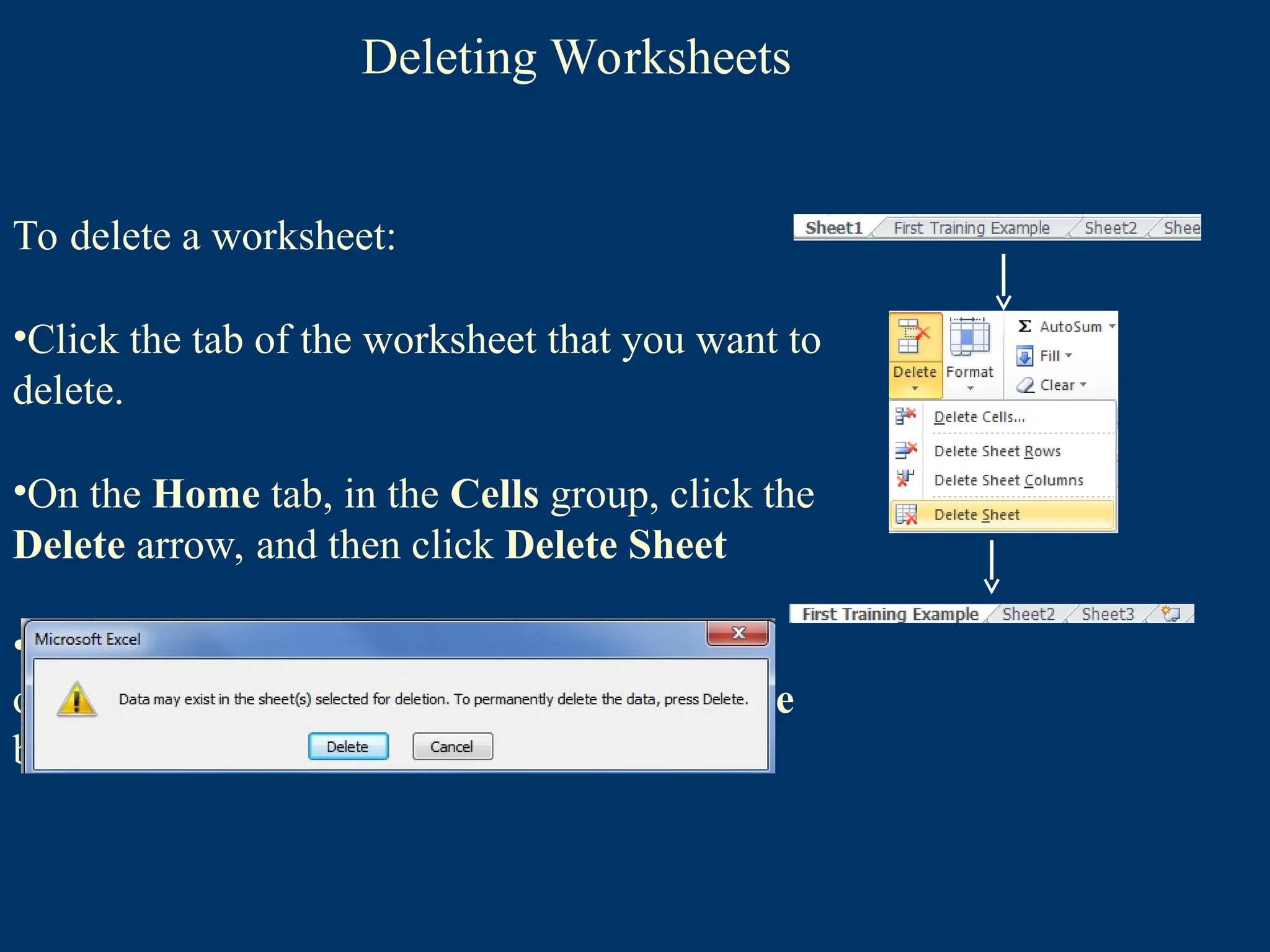
74. Deleting Worksheets
To delete a worksheet:
•Click the tab of the worksheet that you want to
delete.
•On the Home tab, in the Cells group, click the
Delete arrow, and then click Delete Sheet
•If the worksheet contains data, a dialog box
opens asking you to confirm. Click the Delete
button .

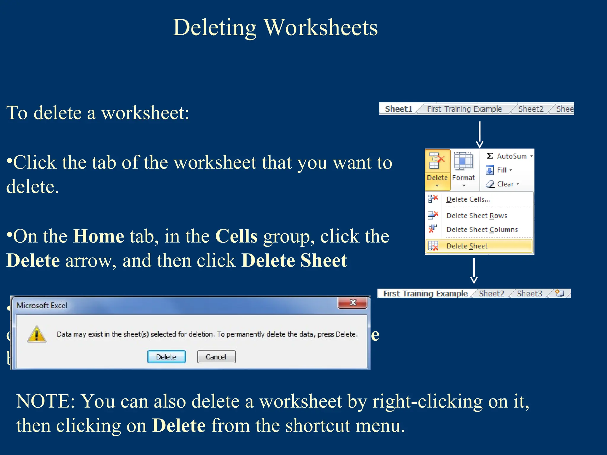
75. Deleting Worksheets
To delete a worksheet:
•Click the tab of the worksheet that you want to
delete.
•On the Home tab, in the Cells group, click the
Delete arrow, and then click Delete Sheet
•If the worksheet contains data, a dialog box
opens asking you to confirm. Click the Delete
button .
NOTE: You can also delete a worksheet by right-clicking on it,
then clicking on Delete from the shortcut menu.

76. Moving Worksheets
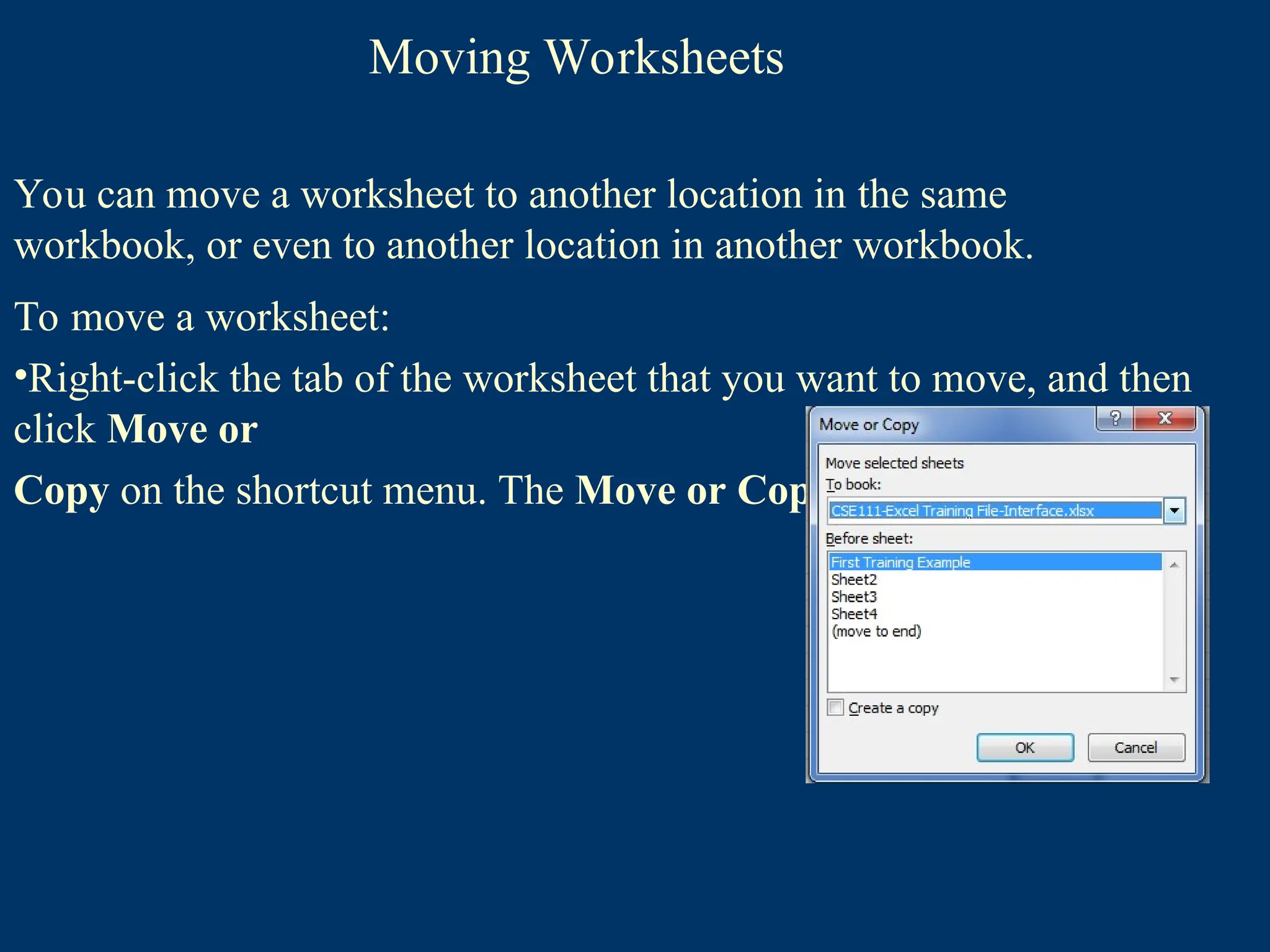
You can move a worksheet to another location in the same
workbook, or even to another location in another workbook.

77. Moving Worksheets
You can move a worksheet to another location in the same
workbook, or even to another location in another workbook.
To move a worksheet:
•Right-click the tab of the worksheet that you want to move, and then
click Move or
Copy on the shortcut menu. The Move or Copy dialog box opens

78. Moving Worksheets
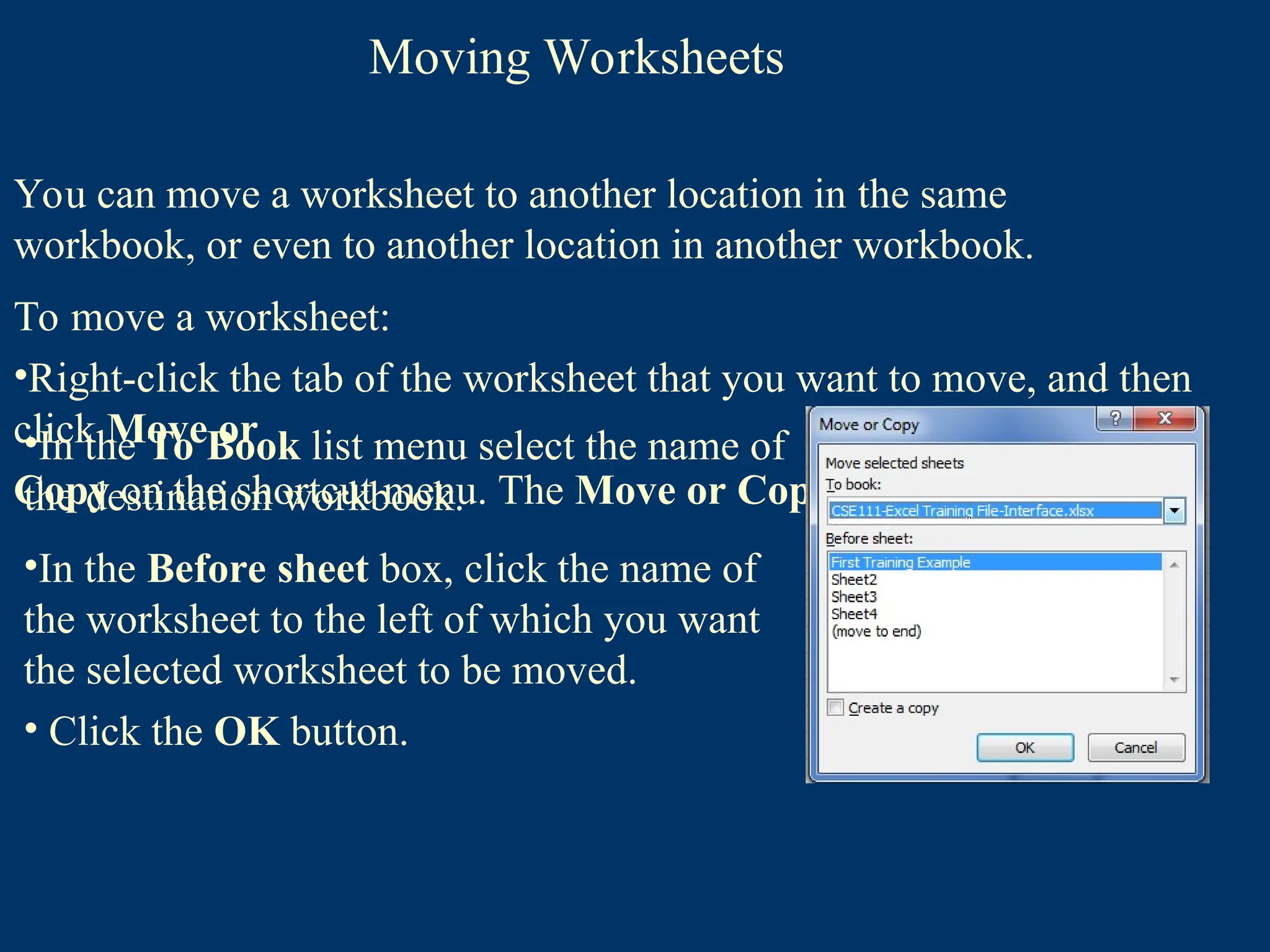
You can move a worksheet to another location in the same
workbook, or even to another location in another workbook.
To move a worksheet:
•Right-click the tab of the worksheet that you want to move, and then
click Move or
Copy on the shortcut menu. The Move or Copy dialog box opens
•In the To Book list menu select the name of
the destination workbook.
•In the Before sheet box, click the name of
the worksheet to the left of which you want
the selected worksheet to be moved.
• Click the OK button.

79. Moving Worksheets
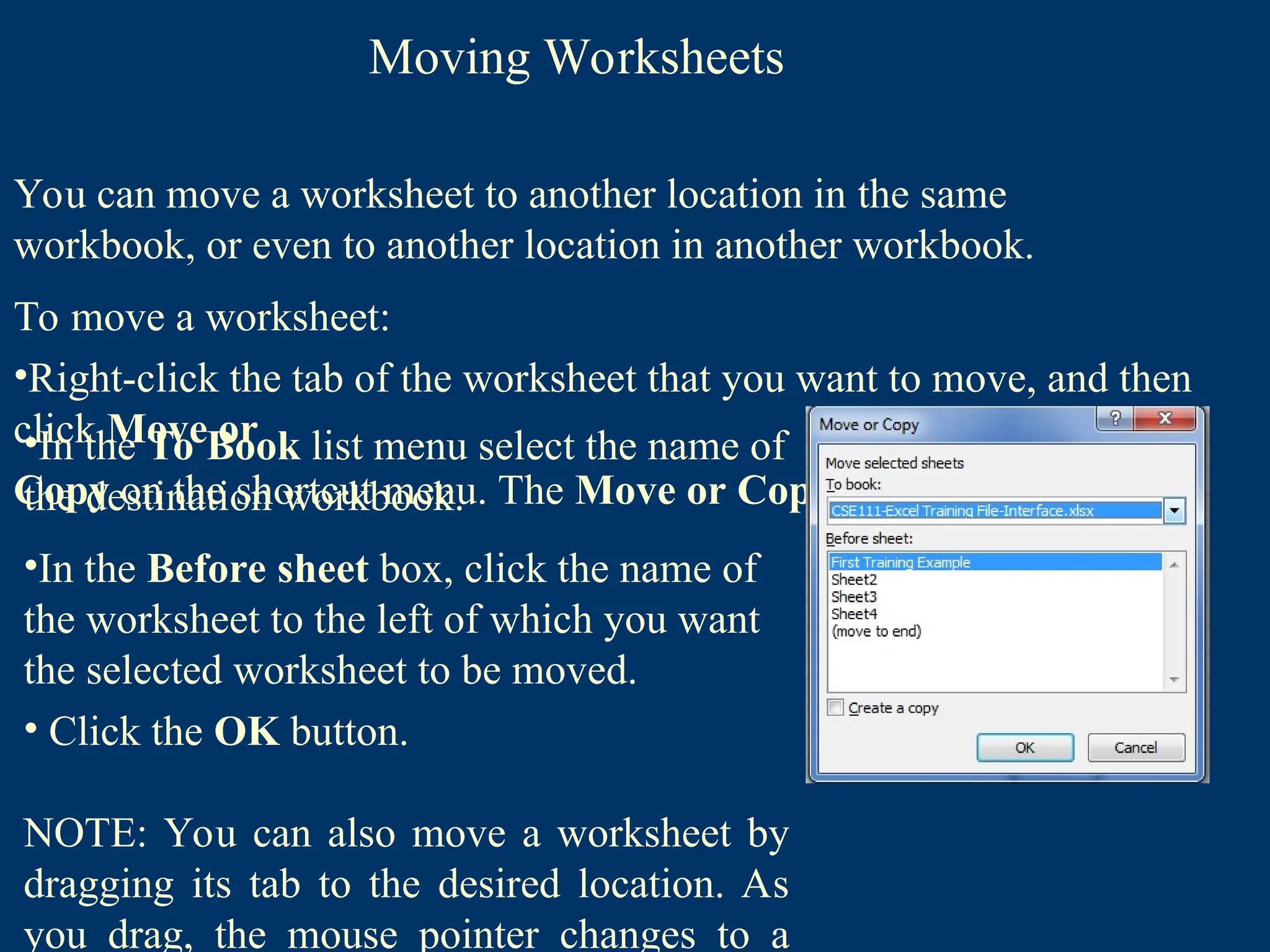
You can move a worksheet to another location in the same
workbook, or even to another location in another workbook.
To move a worksheet:
•Right-click the tab of the worksheet that you want to move, and then
click Move or
Copy on the shortcut menu. The Move or Copy dialog box opens
•In the To Book list menu select the name of
the destination workbook.
•In the Before sheet box, click the name of
the worksheet to the left of which you want
the selected worksheet to be moved.
• Click the OK button.
NOTE: You can also move a worksheet by
dragging its tab to the desired location. As
you drag, the mouse pointer changes to a

80. Copying Worksheets
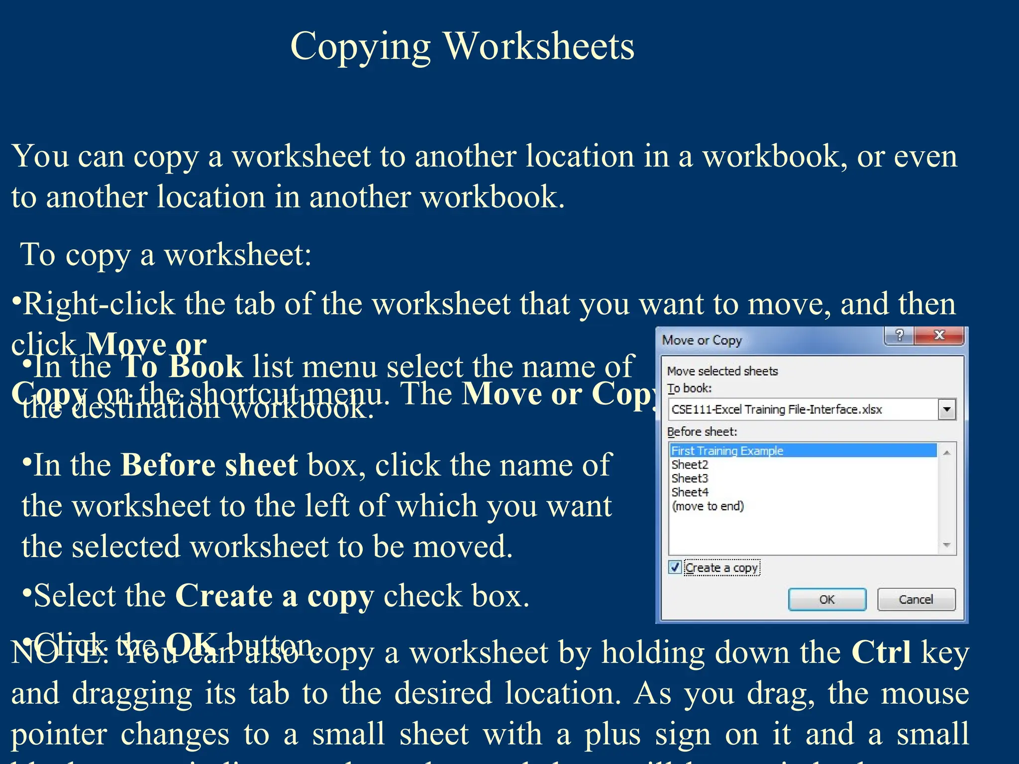
You can copy a worksheet to another location in a workbook, or even
to another location in another workbook.
To copy a worksheet:
•Right-click the tab of the worksheet that you want to move, and then
click Move or
Copy on the shortcut menu. The Move or Copy dialog box opens
•In the To Book list menu select the name of
the destination workbook.
•In the Before sheet box, click the name of
the worksheet to the left of which you want
the selected worksheet to be moved.
•Select the Create a copy check box.
•Click the OK button.
NOTE: You can also copy a worksheet by holding down the Ctrl key
and dragging its tab to the desired location. As you drag, the mouse
pointer changes to a small sheet with a plus sign on it and a small

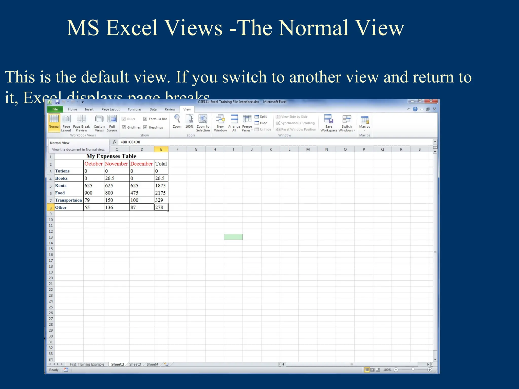
81. MS Excel Views -The Normal View
This is the default view. If you switch to another view and return to
it, Excel displays page breaks.

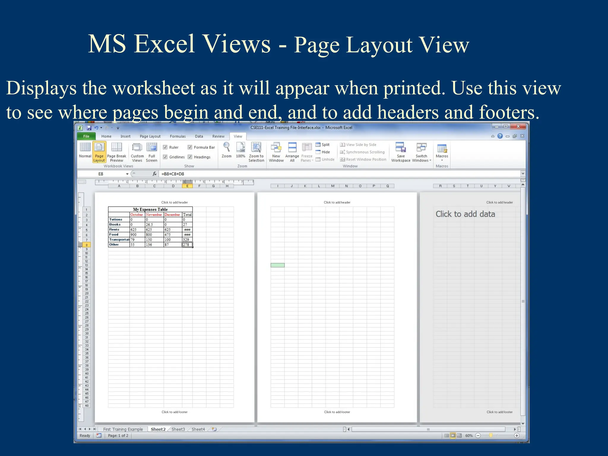
82. MS Excel Views - Page Layout View
Displays the worksheet as it will appear when printed. Use this view
to see where pages begin and end, and to add headers and footers.

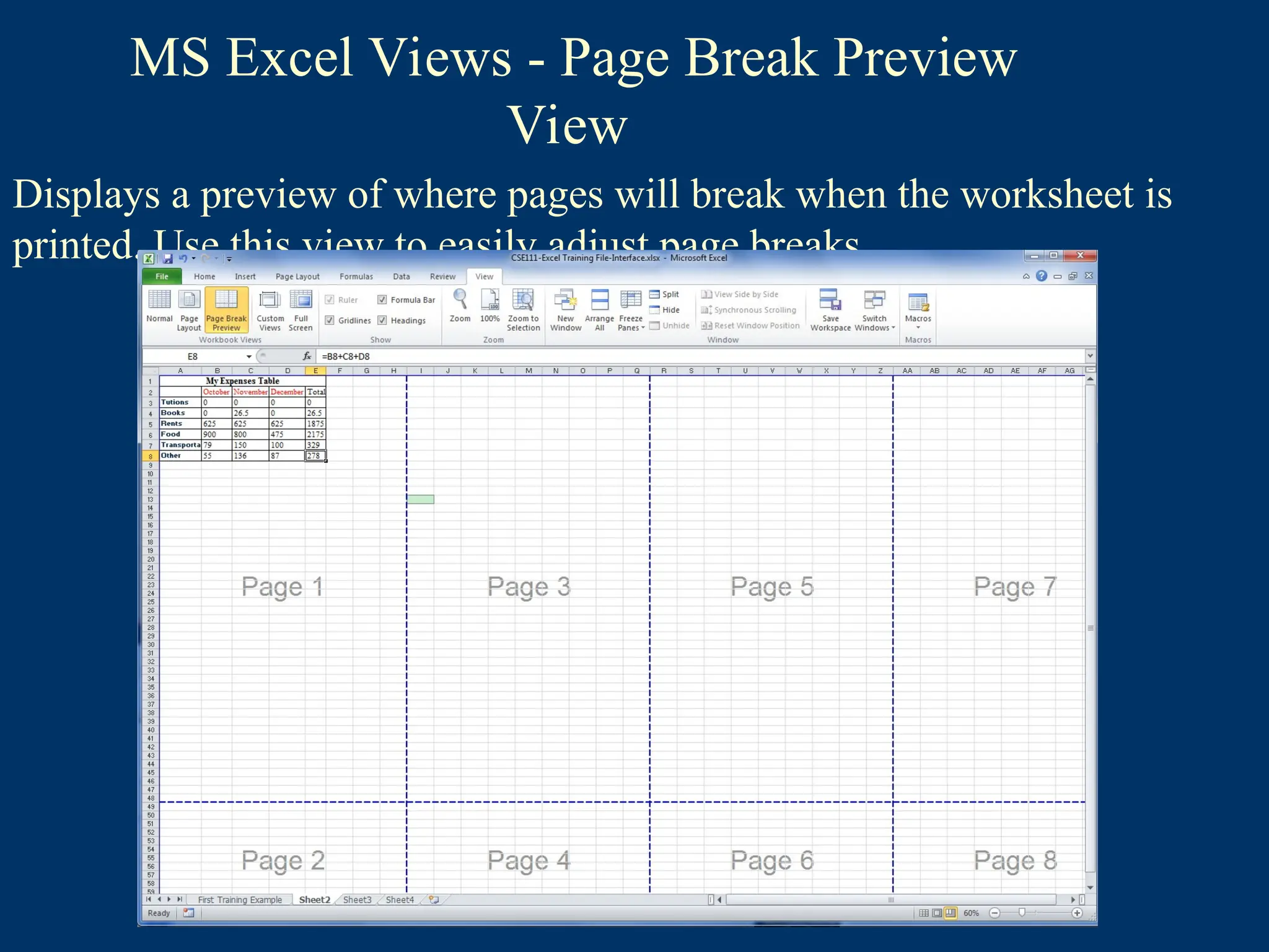
83. MS Excel Views - Page Break Preview
View
Displays a preview of where pages will break when the worksheet is
printed. Use this view to easily adjust page breaks.

84. MS Excel Views - Custom Views
Allows you to save a set of display and print settings as a custom
view, and then apply it.

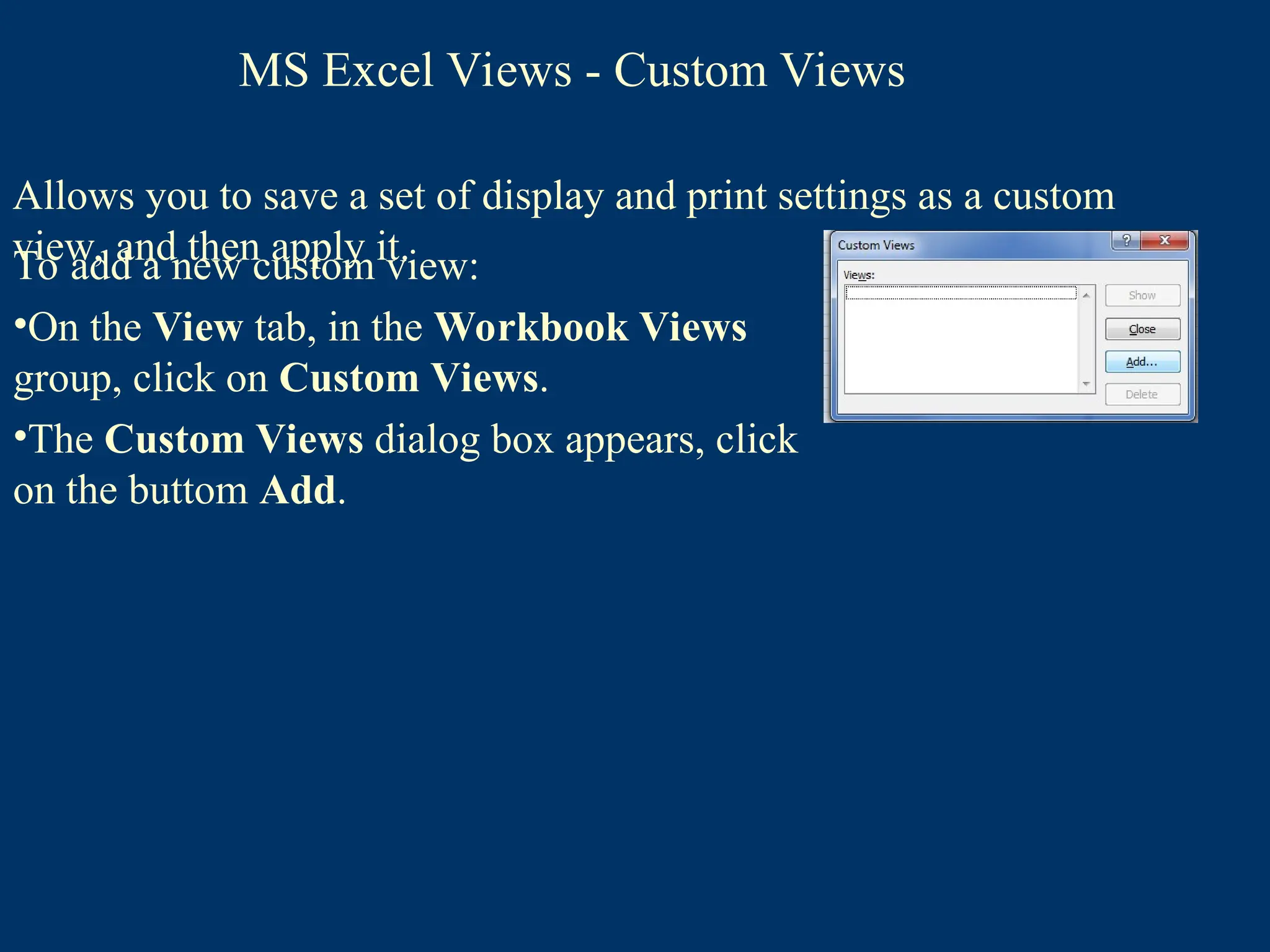
85. Allows you to save a set of display and print settings as a custom
view, and then apply it.
To add a new custom view:
•On the View tab, in the Workbook Views
group, click on Custom Views.
•The Custom Views dialog box appears, click
on the buttom Add.
MS Excel Views - Custom Views

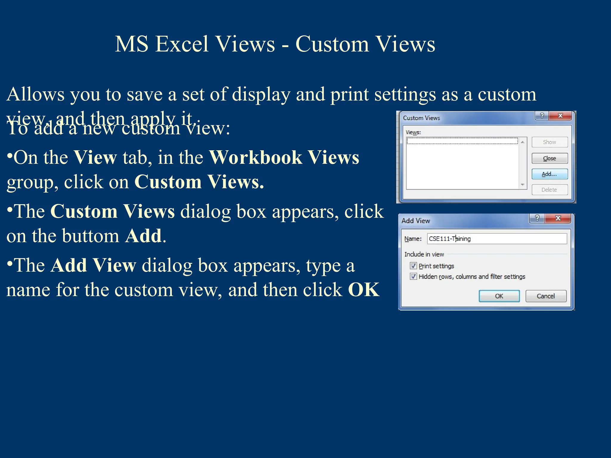
86. Allows you to save a set of display and print settings as a custom
view, and then apply it.
To add a new custom view:
•On the View tab, in the Workbook Views
group, click on Custom Views.
•The Custom Views dialog box appears, click
on the buttom Add.
•The Add View dialog box appears, type a
name for the custom view, and then click OK
MS Excel Views - Custom Views

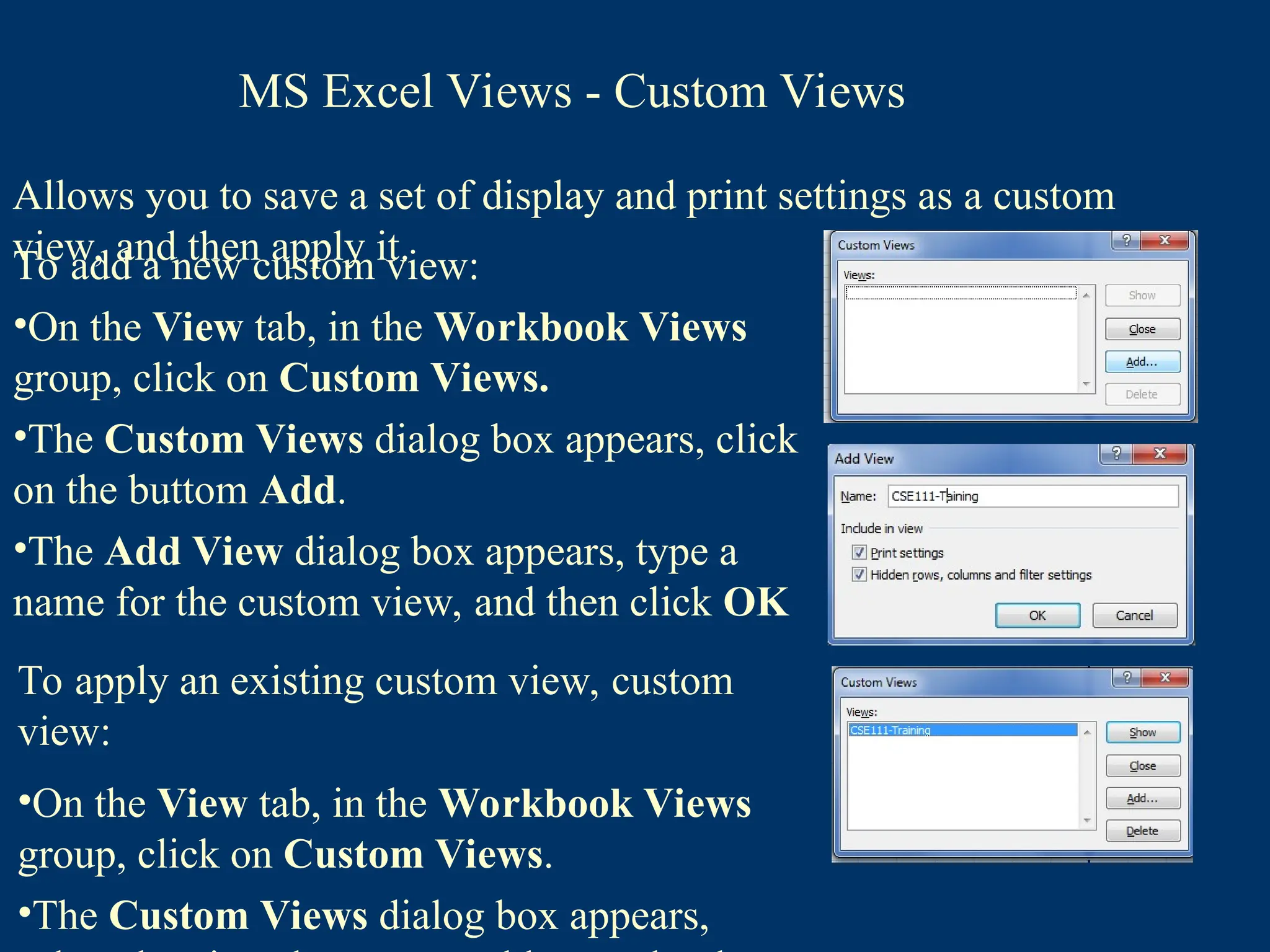
87. Allows you to save a set of display and print settings as a custom
view, and then apply it.
To add a new custom view:
•On the View tab, in the Workbook Views
group, click on Custom Views.
•The Custom Views dialog box appears, click
on the buttom Add.
•The Add View dialog box appears, type a
name for the custom view, and then click OK
To apply an existing custom view, custom
view:
•On the View tab, in the Workbook Views
group, click on Custom Views.
•The Custom Views dialog box appears,
MS Excel Views - Custom Views

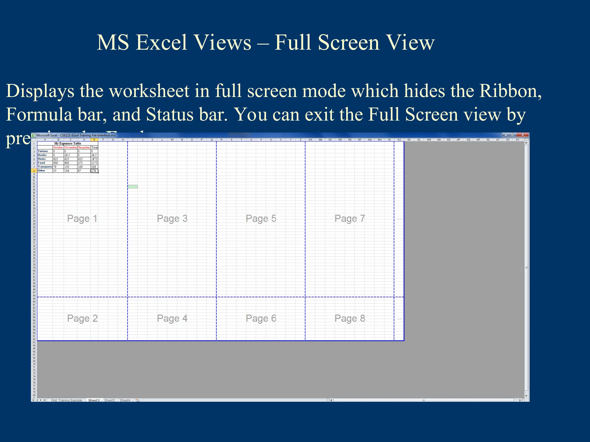
88. Displays the worksheet in full screen mode which hides the Ribbon,
Formula bar, and Status bar. You can exit the Full Screen view by
pressing the Esc key.
MS Excel Views – Full Screen View

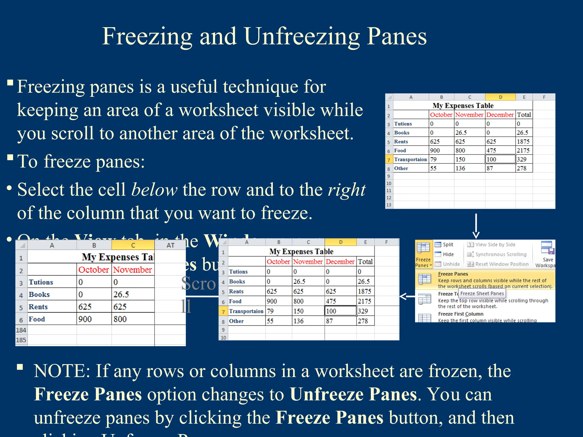
89. Freezing and Unfreezing Panes
Freezing panes is a useful technique for
keeping an area of a worksheet visible while
you scroll to another area of the worksheet.

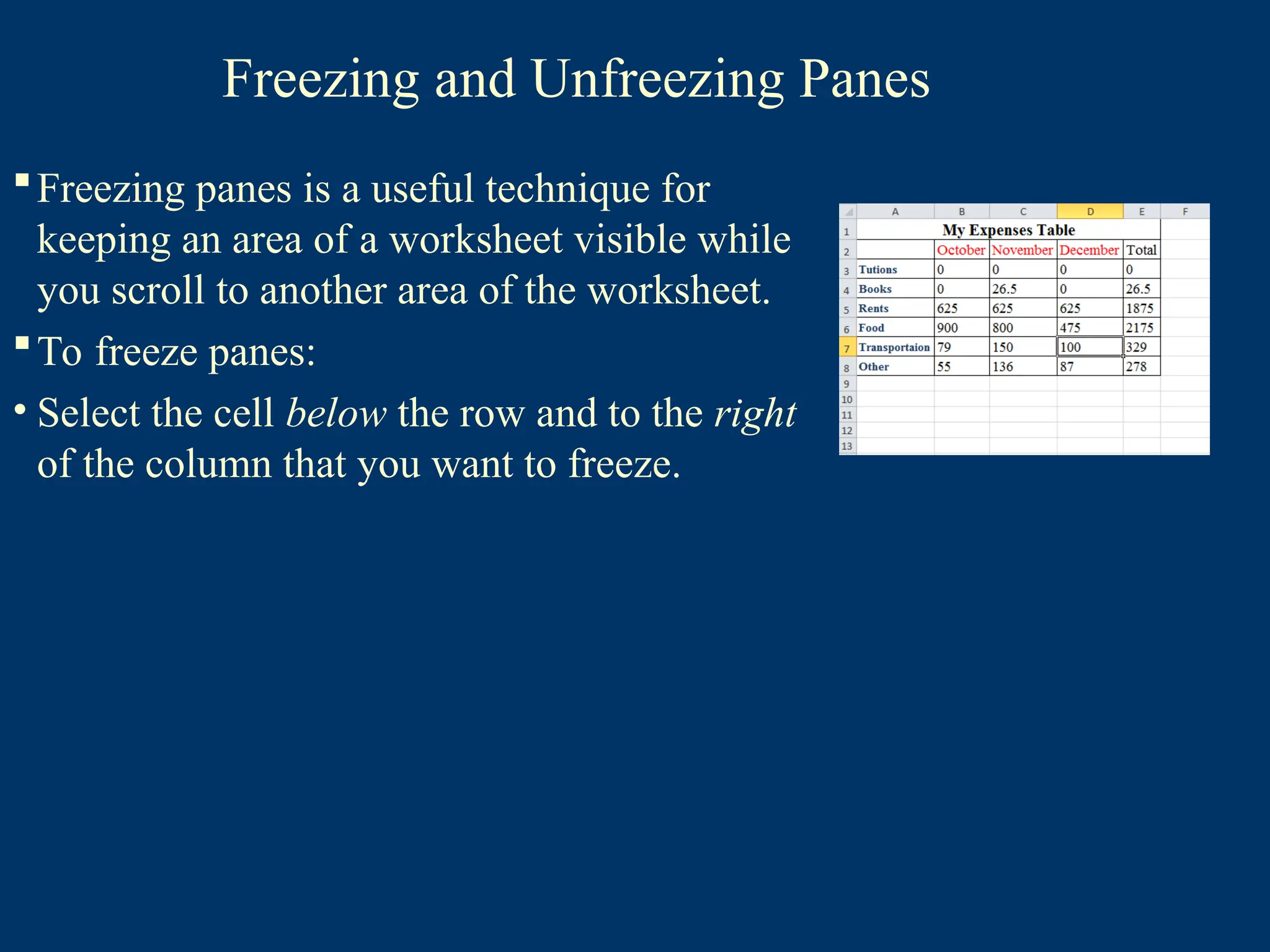
90. Freezing and Unfreezing Panes
Freezing panes is a useful technique for
keeping an area of a worksheet visible while
you scroll to another area of the worksheet.
To freeze panes:
• Select the cell below the row and to the right
of the column that you want to freeze.

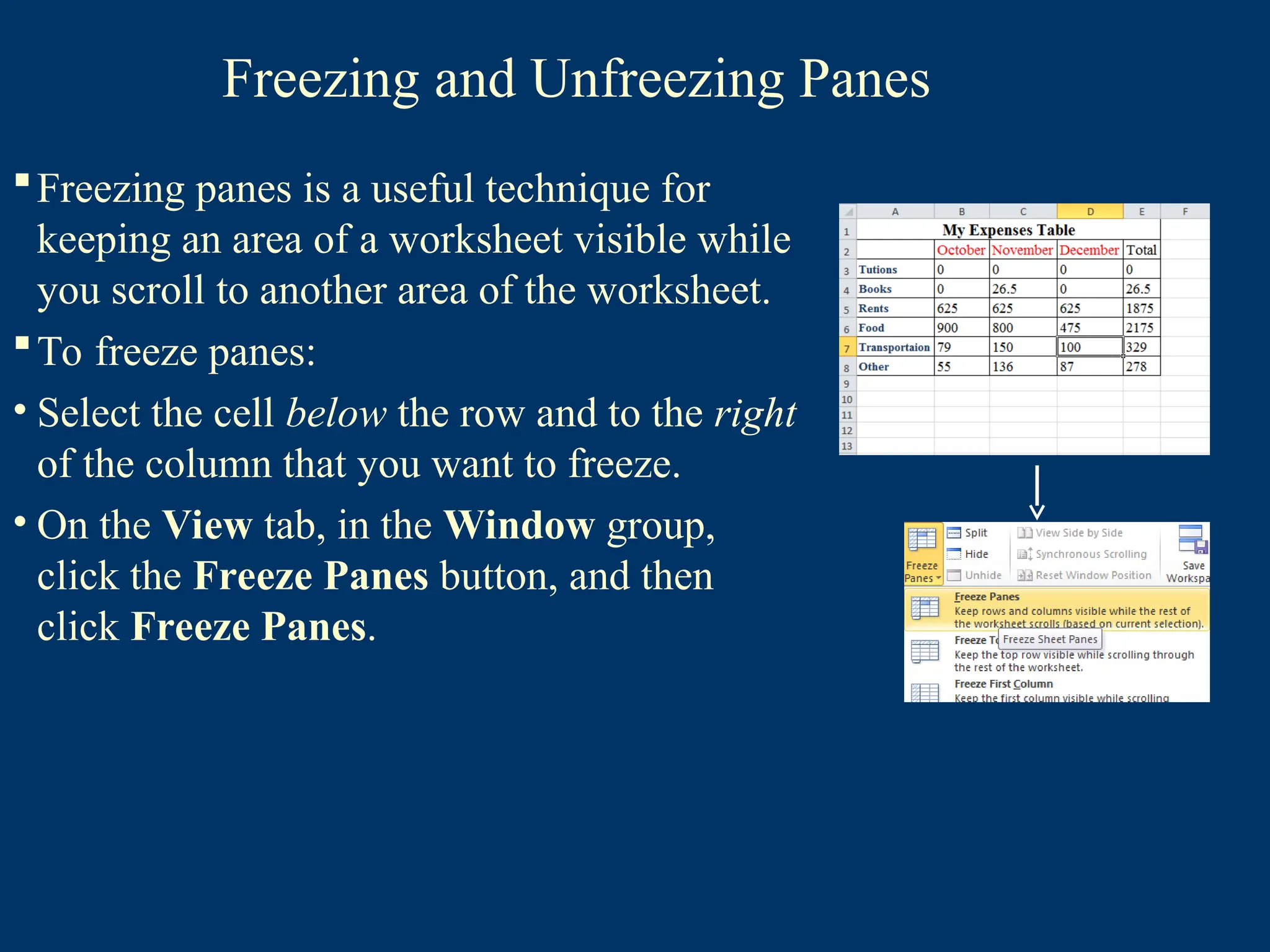
91. Freezing and Unfreezing Panes
Freezing panes is a useful technique for
keeping an area of a worksheet visible while
you scroll to another area of the worksheet.
To freeze panes:
• Select the cell below the row and to the right
of the column that you want to freeze.
• On the View tab, in the Window group,
click the Freeze Panes button, and then
click Freeze Panes.

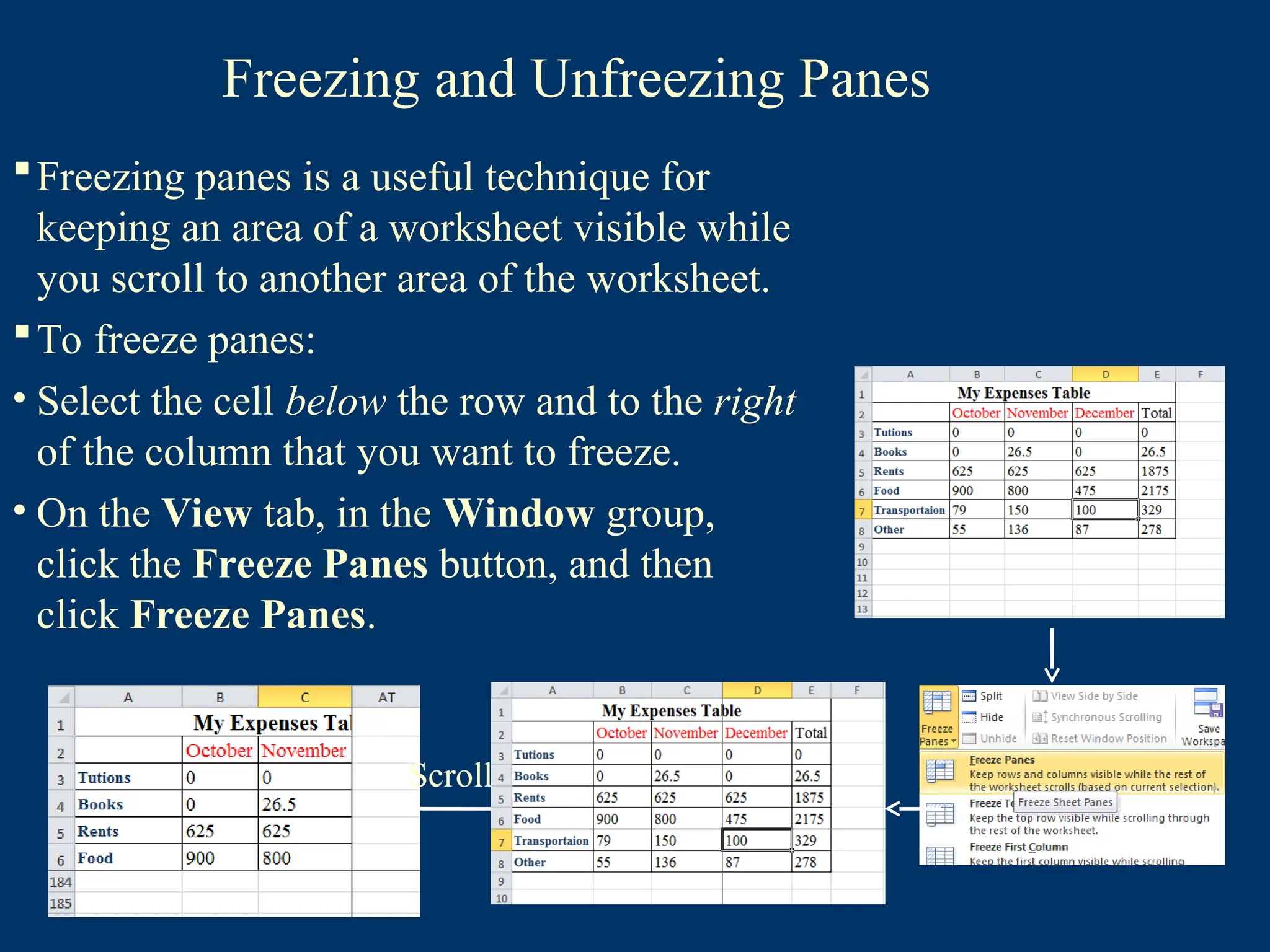
92. Freezing and Unfreezing Panes
Freezing panes is a useful technique for
keeping an area of a worksheet visible while
you scroll to another area of the worksheet.
To freeze panes:
• Select the cell below the row and to the right
of the column that you want to freeze.
• On the View tab, in the Window group,
click the Freeze Panes button, and then
click Freeze Panes.
Scroll

93. Freezing and Unfreezing Panes
Freezing panes is a useful technique for
keeping an area of a worksheet visible while
you scroll to another area of the worksheet.
To freeze panes:
• Select the cell below the row and to the right
of the column that you want to freeze.
• On the View tab, in the Window group,
click the Freeze Panes button, and then
click Freeze Panes. Scro
ll
 NOTE: If any rows or columns in a worksheet are frozen, the
Freeze Panes option changes to Unfreeze Panes. You can
unfreeze panes by clicking the Freeze Panes button, and then

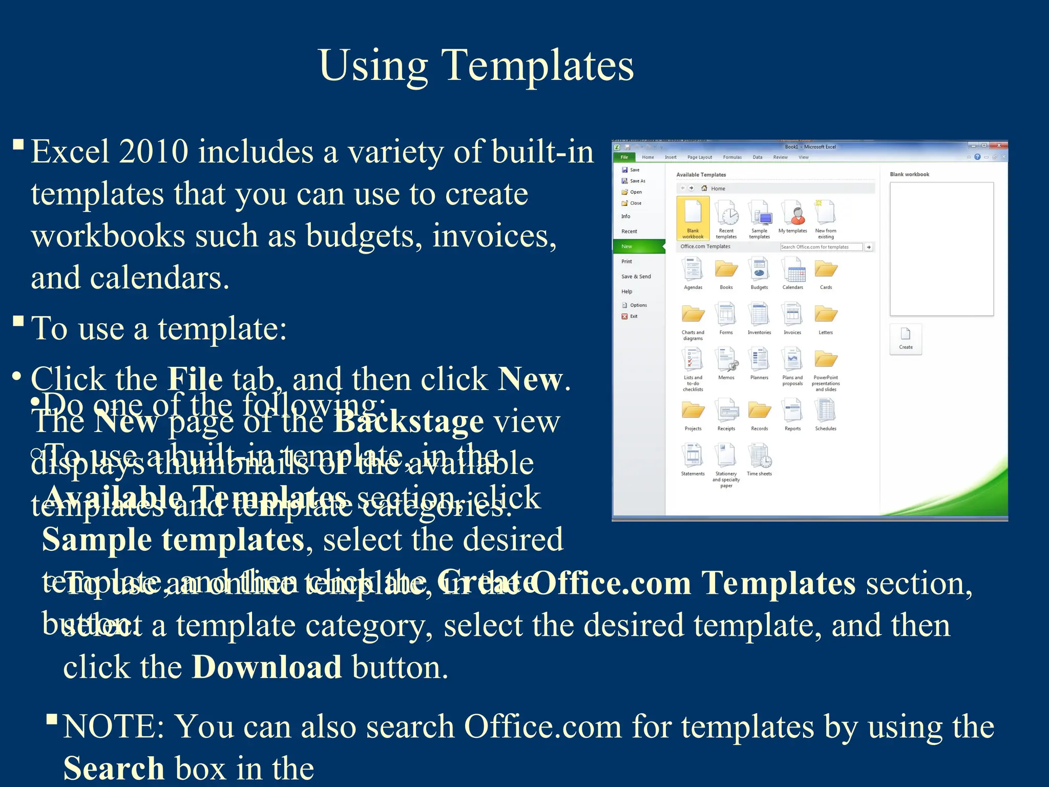
94. Using Templates
Excel 2010 includes a variety of built-in
templates that you can use to create
workbooks such as budgets, invoices,
and calendars.
To use a template:
• Click the File tab, and then click New.
The New page of the Backstage view
displays thumbnails of the available
templates and template categories.
•Do one of the following:
oTo use a built-in template, in the
Available Templates section, click
Sample templates, select the desired
template, and then click the Create
button.
o To use an online template, in the Office.com Templates section,
select a template category, select the desired template, and then
click the Download button.
NOTE: You can also search Office.com for templates by using the
Search box in the