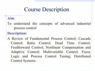
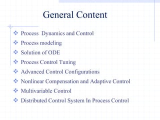
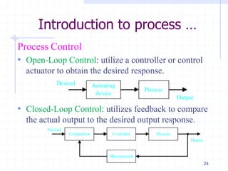
This document provides an overview of a course on advanced process control fundamentals. The course aims to understand concepts of advanced industrial process control. Topics covered include process dynamics and control, process modeling, solution of differential equations, advanced control configurations, nonlinear compensation, multivariable control, and distributed control systems. Prerequisites for the course are several introductory control systems courses. The first lecture provides an introduction to process dynamics and control, including modeling a process, process control objectives, and the first order dynamics of processes. Process modeling involves formulating material and energy balances, developing constitutive equations, and ensuring the appropriate degrees of freedom.
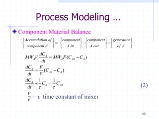
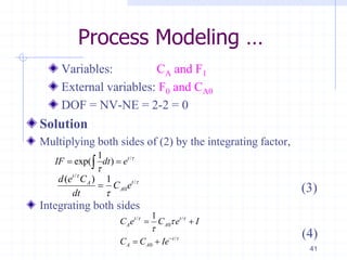
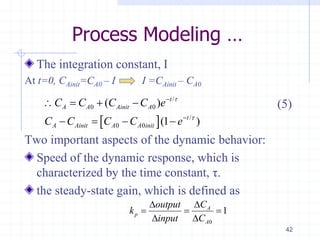
![Process Modeling …
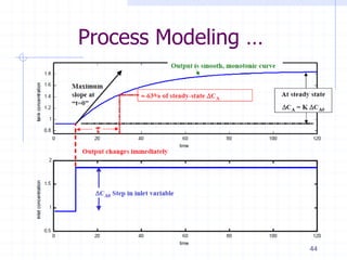
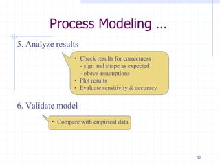
Results Analysis
43
Time
from step
Percent of final steady-
state change in output
0 0
T 63.2
2T 86.2
3T 95
4T 98.2
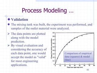
The goal statement
involves determining
the time until 90 % of
the change in outlet
concentration has
occurred.
This time can be calculated by setting
CA = CAinit + 0.9(CA0 - CAinit) in eqn. (5) and solving
Ainit A0
Ainit A0
0.1[ ]
ln (24.7)( 2.3) 56.8min
C C
t
C C
](https://image.slidesharecdn.com/ep-5512lecture-01-190313233546/85/Ep-5512-lecture-01-43-320.jpg)