siajfiosajoifjsdaioj

1. 6 1 CHAPTER 1
These discrete-state control systems are often implemented using specialized
computer-based equipment called programmable logic controllers (PLCs). Chapter 8
will present an ftin-depth consideration of discrete-state control systems and PLCs.
1.3 PROCESS-CONTROL BLOCK DIAGRAM
To provide a practical, working description of process control, it is useful to describe
the elements and operations involved in more generic terms. Such a description should
be in-dependent of a particular application (such as the example presented in the
previous sec-tion) and thus be applicable to all control situations. A model may be
constructed usingblocks to represent each distinctive element. The characteristics of
control operation thenmay be developed from a consideration of the properties and
interfacing of these elements.
Numerous models have been employed in the history of process-control description;
wewill use one that seems most appropriate for a description of modem and
developing technology of process control.
1.3.1 Identification of Elements
The elements of a process-control system are defined in terms of separate functional
parts of the system. The following paragraphs define the basic elements of a process-control
system and relate them to the example presented in Section 1.2.
Process In the previous example, the flow of liquid in and out of the tank, the
tank itself, and the liquid all constitute a process to be placed under control with
respect to the fluid level. In general, a process can consist of a complex assembly of
phenomena that relate to some manufacturing sequence. Many variables may be
involved in such a process, and it may be desirable to control all these variables at the
same time. There are single-variable processes, in which only one variable is to be
controlled, as well as multivariable processes, in which many variables, perhaps
interrelated, may require regulation. The process is often also called the plant.

2. Measurement Clearly, to effect control of a variable in a process, we must have
information about the variable itself. Such information is found by measuring the
variable. In general, a measurement refers to the conversion of the variable into some
corresponding analog of the variable, such as a pneumatic pressure, an electrical
voltage or current, or a digitally encoded signal. A sensor is a device that performs the
initial measurement and energy conversion of a variable into analogous digital,
electrical, or pneumatic information.
Further transformation or signal conditioning may be required to complete the
measurement function. The result of the measurement is a representation of the
variable value in some form required by the other elements in the process-control
operation.
In the system shown in Figure 1.3, the controlled variable is the level of liquid in
the tank. The measurement is performed by some sensor, which provides a signal, s, to
the controller. In the case of Figure 1.2, the sensor is the sight tube showing the level
to the human operator as an actual level in the tank.
The sensor is also called a transducer. However, the word sensor is preferred for
the initial measurement device because "transducer" represents a device that converts
any signal from one form to another. Thus, for example, a device that converts a
voltage into a proportional current would be a transducer. In other words, all sensors
are transducers, but not all transducers are sensors.
Error Detector In Figure 1.2, the human looked at the difference between the
actual level, h, and the setpoint level, H, and deduced an error. This error has both a
magnitude and polarity. For the automatic control system in Figure 1.3, this same kind
of error determination must be made before any control action can be taken by the
controller. Al-dxxish the error detector is often a physical part of the controller device,
it is important to keep a clear distinction between the two.
Controller The next step in the process-control sequence is to examine the error and
docmuoe what action, if any, should be taken. This part of the control system has

3. many such as compensator ox filter, but controller is the most common. The
evaluation may performed by an operator (as in the previous example), by electronic
signal processing, by : signal processing, or by a computer. In modem control
systems, the operations of typically performed by microprocessor-based computers.
The controller of both a measured indication of the controlled variable and a
representation value of the variable. expressed in the same terms as the measured
value. The of the variable, you will recall, is referred to as the setpoint. Evaluation
con-: the action required to drive the controlled variable to the setpoint value.
Control Element The final element in the process-control operation is the device »a
direct influence on the process; that is. it provides those required changes in ; M»
bna^ M lo Itae setpouu. This element accepts an input from the ie proportional
operation performed on the .ife« is the valve that adjusts the outflow BtfhawBcn the
controller output and the Summing This block diagram of a control loop defines all
the basic elements and signals involved. Figure 1.6 shows how a physical control
system is represented as a block diagram.n The physical system for control of flow
through a pipe is shown in Figure 1.6. Variation of flow through an obstruction (the
orifice plate) produces a pressure-difference variation across the obstruction. This
variation is converted to the standard signal range of 3 to 15 psi. The P/I converter
changes the pressure to a 4- to 20-mA electric current, which is sent to the controller.
The controller outputs a 4- to 20-mA control signal to signify the cor- rect valve
setting to provide the correct flow. This current is converted to a 3- to 15-psi pres-sure
signal by the VP converter and applied to a pneumatic actuator. The actuator then
adjusts the valve setting.
Figure 1.6
shows how all the control system operations are condensed to the stan- dard
block diagram operations of measurement, error detection, controller, and final con-trol
element.
The purpose of a block diagram approach is to allow the process-control system
to be analyzed as the interaction of smaller and simpler subsystems. If the

4. characteristics of each element of the system can be determined, then the
characteristics of the assembled system can be established by an analytical marriage of
these subsystems. The historical development of the system approach in technology
was dictated by this practical aspect: first, to specify the characteristics desired of a
total system, and then, to delegate the development of subsystems that provide the
overall criteria.
It becomes evident that the specification of a process-control system to regulate a
variable, c, within specified limits and with specified time responses, determines the
char- acteristics the measurement system must possess. This same set of system
specifications is reflected in the design of the controller and control element.
Prom this concept, we conclude that the analysis of a process-control system re-quires
an understanding of the overall system behavior and the reflection of this
behavior in the properties of the system elements. Most people find that an
understanding of
1.4 CONTROL SYSTEM EVALUATION
A process-control system is used to regulate the value of some process variable. When
such a system is in use, it is natural to ask, How well is it working? This is not an easy
question to answer, because it is possible to adjust a control system to provide
different kinds of response to errors. This section discusses some methods for
evaluating how well the system is working.
The variable used to measure the performance of the control system is the error.
e(t), which is the difference between the constant setpoint or reference value, r, and
the controlled variable, c(f).
e(t)=r-c(t} (1.1)'
Since the value of the controlled variable may vary in time, so may the error. (Note
that in a servomechanism, the value of r may be forced to vary in time also.)

5. Control System Objective In principle, the objective of a control system is to make
the error in Equation (1.1) exactly zero, but the control system responds only to errors
(i.e., when an error occurs, the control system takes action to drive it to zero).
Conversely, if the error were zero and stayed zero, the control system would not be
doing anything and would not be needed in the first place. Therefore, this objective
can never be perfectly achieved, and there will always be some error. The question of
evaluation becomes one of how large the error is and how it varies in time.
A practical statement of control system objective is best represented by three
requirements:
1. The system should be stable.
2. The system should provide the best possible steady-state regulation.
3. The system should provide the best possible transient regulation.
1.4.1 Stability
The purpose of the control system is to regulate the value of some variable. This
requires that action be taken on the process itself in response to a measuremqpt of the
variable. If this is not done correctly, the control system can cause the process to
become unstable. In fact, the more tightly we try to control the variable, the greater the
possibility of instability.
Figure 1.7 shows that, prior to turning on a control system, the controlled variable
drifts in a random fashion and is not regulated. After the control system is turned on,
the -variable is forced to adopt the setpoint value, and all is well for awhile. Notice
that some time later, however, the variable begins to exhibit growing oscillations of
value—that is, an instability. This occurs even though the control system is still
connected and operational; in fact, it occurs because the system is connected and
operational.

6. The first objective, then, simply means that the control system must be designed
and adjusted so that the system is stable. Typically, as the control system is adjusted to
give belter control, the likelihood of instability also increases.
Steady-State Regulation
The objective of the best possible steady-state regulation simply means that the
steady- state error should be a minimum. Generally, when a control system is
specified, there will be some allowable deviation, ±Ac, about the setpoint. This means
that variations of the variable within this band are expected and acceptable. External
influences that tend to cause drifts of the value beyond the allowable deviation are
corrected by the control system.
For example, a process-control technologist might be asked to design and
implement a control system to regulate temperature at 150°C within ±2°C. This means
the setpoint is to be 150°C, but the temperature may be allowed to vary within the
range of 148° to 152°C.
1.4.3 Transient Regulation
What happens to the value of the controlled variable when some sudden transient
event occurs that would otherwise cause a large variation? For example, the setpoint
could change. Suppose the setpoint in the aforementioned temperature case were
suddenly changed to IWC. Transient regulation specifies how the control system
reacts to bring the temperature to this new setpoint.
Another type of transient influence is a sudden change of some other process
variable. The controlled variable depends on other process variables. If one of them
suddenly changes value, the controlled variable may be driven to change also, so the
control system acts to minimize the effect. This is called transient response.
1.4.4 Evaluation Criteria
The question of how well the control system is working is thus answered by (1)
ensuring stability, (2) evaluating steady-state response, and (3) evaluating the response

7. to set point changes and transient effects. There are many criteria for gauging the
response. In general, the term tuning is used to indicate how a process-control loop is
adjusted to provide the best control. This topic is covered in more detail in Chapter
12.
FIGURE 1.8
One of the measures of control system performance is how the system responds to
changes of setpoint or a transient disturbance. Setpoint change Transient occurs
Damped Response One type of criterion requires that thecontrolled variable ex-hibit
a response such as that shown in Figure 1.8 for excitations of both setpoint
changes and transient effects. Note that the error is of only one polarity (i.e., it never
oscillates about the set point). For this case, measures of quality are the duration, to, of
the excursion and, for the transient, the maximum error, e^, for a given input. The
duration is usually defined as the time taken for the controlled variable to go from
10% of the change to 90% of the change following a setpoint change. In the case of a
transient, the duration is often defined as the time from the start of the disturbance
until the controlled variable is again within 4% of the reference.
Different tuning will provide different values of £„„ and tp for the same
excitation. It is up to the process designers to decide whether the best control is larger
duration with smaller peak error, or vice versa, or something in between.
Cyclic Response Another type of criterion applies to those cases in which the
response to a setpoint change or transient is as shown in Figure 1.9. Note that the
controlled vanable oscillates about the setpoint. In this case, the parameters of interest
are the maximum error.
E max and the duration, ty, also called the settling time. The duration is measured
from the time when the allowable error is first exceeded to the time when it falls
within the allowable error and stays.

8. The nature of the response is modified by adjusting the control loop parameters,
which is called tuning. There may be large maximum error but short duration or long
duration with small maximum error, and everything in between.
A number of standard cyclic tuning criteria are used. Two common types are
minimum area and quarter amplitude. In minimum area, the tuning is adjusted until
the net area under the error-time curve is a minimum, for the same degree of
excitation (setpoint change or transient). Figure 1.10 shows the area as a shaded part
of the curve. Analytically, this is given by
A ^ {e(t)dt = minimum (1.2)
The quarter-amplitude criterion, shown in Figure 1.10, specifies that the
amplitude of each peak of the cyclic response be a quarter of the preceding peak.
Thus, a2 = fli/4,fl3 = a-i/4, and so on.
all pneumatic and has a flow transmitter (FT/302), a flow controller (FC/302), and a
flow recorder (FR/302), which is located in the control room. Note that the sensor
actually measures pressure and that the flow is proportional to the square root of
pressure. Therefore, a square-root extractor is indicated following the flow transmitter.
The flow recorder charts variations of flow rate for an operator.
Figure 1.26 shows a flow loop under computer control. This flow control
computer. FC 220, is located in the field (i.e., at the site of control). This is an all -
electrical loop that inputs a 4- to 20-mA signal for flow measurement and outputs a 4-
to 20-mA signal to the control valve, FV/220. A level transmitter, LT/220, provides
input to a computer, LC/220, which is located in the control room. The output of this
computer is the setpoint of the flow loop. Finally, a PLC, shown as a diamond within
a box, YIC/225, can open or close the tank drain valve.
Other Symbols Figures 1.25 and 1.26 also show the symbols for several other el-ements
associated with the control systems and plants. For example, the control valves
are often identified in terms of what they control. In Figure 1.25, the steam valve is

9. labeled TV/301 to indicate that it is for temperature control even though it is actually
controlling steam flow.
Both figures show an orifice plate used to measure flow through a pipe. The valve
actuator shown in Figure 1.26 with the PLC indicates it is spring-loaded and
electrically actuated. Appendix 5 shows more P&ID symbols defined by the S5.1
standard and some expanded information about its application.
1.7 SENSOR TIME RESPONSE
The static transfer function of a process-control loop element specifies how the output
is related to the input if the input is constant. An element also has a time dependence
that specifies how the output changes in time when the input is changing in time. It is
independent from the static transfer function. This dynamic transfer function, which is
independent from the staticitransfer function, is often simply called the time response.
It is particularly important for sen-Isors because they are the primary element for
providing knowledge of the controlled variable!
value. This section will discuss the two most common types of sensor time responses.
Figure 1.27 shows a sensor that produces an output, b(t), as a function of the
input. •(()• The static transfer function determines the output when the input is not
changing ml time. To specify the time response, the nature of the time variation in
output, b(t), is givea|
FIGURE 1.27
The dynamic transfer function specifies how a sensor output varies when the input
changes instantaneously in time (i.e., a step change).
FIGURE 1.28
Characteristic first-order exponential time response of a sensor to a step change of
input.

10. when the input exhibits a step change as shown. Note that at t = 0 the input to the
sensor is suddenly changed from an initial value, c,, to a final value, Cf. If the sensor
were perfect, its output would be determined by the static transfer function to be &,
before t = 0 and bf after / = 0. However, all sensors exhibit some lag between the
output and the input and some characteristic variation in time before settling on the
final value.
1.7.1 First-Order Response
The simplest time response is shown in Figure 1.28 as the output change in time
following a step input as in Figure 1.27. This is called first order because, for all
sensors of this type, the time response is determined by the solution of a first-order
differentialequation.
A general equation can be written for this response independent of the sensor, the
variable being measured, or the static transfer function. The equation gives the sensor
output as a function of time following the step input (i.e., it traces the curve of Figure
1.28 in time):
b(t) = b, + (bf - 6,)[1 -e-^J (1.7)
where b, » initial sensor output from static transfer function and initial input bf =
final sensor output from static transfer function and final input T = sensor time
constant
The sensor output is in error during the transition time of the output from b, to bf.
The actual variable value was changed instantaneously to a new value at t = 0.
Equation (1.7) describes transducer output very well except during the initial time
period—that is, at the start of the response near t = 0. In particular, the actual
transducer response generally starts the change with a zero slope, and Equation (1.7)
predicts a finite starting slope.
Time Constant The time constant, T, is part of the specification of the sensor. Its
significance can be seen by writing Equation (1.7) as follows

11. b(t) - b. = (bf - b.-^l - e-^} <as
In this equation, the quantity on the left is the change in output as a function of time,
whereas (6y - b,) is the total change that will occur. Thus, the square-bracketed term in
Equation (1.8) is the fraction of total change as a function of time.
Suppose we wish to find the change that has occurred at a time numerically equal
to T. Then we set t = T in Equation (1.8) and find
b(T)-b.=(^-b,)[l-e-1! (1.9)
b^ - bt= 0.6?>l(b^ - b^
Thus, we see that one time constant represents the time at which the output NATO o&
changed by approximately 63% of the total change.
The time constant T is sometimes referred to as the 63% time, the response time,
or the e-folding time. For a step change, the output response has approximately
reached its fi- nal value after five time constants, since from Equation (1.8) we find
b(5-r) - b, = 0.993(b/ - b.)
EXAIVIPLE A sensor measures temperature linearly with a static transfer function of
33 mV/°C and has a 1.5-s time constant. Find the output 0.75 s after the input changes
from 20° to 41°C. Find Jl. the error in temperature this represents.
Solution
We first find the initial and final values of the sensor output:
6, = (33mV/°C)(20°C)
b, =660mV
bf= (33mV/°C)(41°C)
bf = 1353 mV

12. Now,
b(t) - b, + {bf - b,)[l - e-^
&(0.75) = 660 + (1353 - 660) [1 - e^-75^5]
&(0.75) = 932.7 mV
This corresponds to a temperature of
T 932.7
33 mV/°C
T = 28.3°C
Thus the indicated temperature differs from the actual temperature by - 12.7°C
because of the lag in sensor output. After a time of about five times constants ( -7.5 s)
the sensor out-; put would be about 1.353 V, correctly indicating the actual
temperature of 41°C.
In many cases, the transducer output may be inversely related to the input.
Equatic (1.7) still describes the time response of the element where the final output is
less than ft initial output.
Note that the time response analysis is always applied to the output of the sense
never the input. In Example 1.15 the temperature changed suddenly from 20° to 41°C,
it would be wrong to write equations for the temperature in terms of first -order time
sponse. Il is only the output of the sensor that lagged. Particularly if the sensor output
varies nonlineariy with its input, terrible errors will occur if the time response
equation is applied to the input.
Real-Time Effects The concept of the exponential time response and associated
time constant is based on a sudden discontinuous change of the input value. In the real
world, such instantaneous changes occur rarely, if ever, and thus we have presented a

13. worst-case situation in the time response. In general, a sensor shouid be able to track
any changes in the physical dynamic variable in a time less than one time constant.
1,7.2 Second-Order Response
In some sensors, a step change in [he input causes the output to osciliate for a short
period of time before settling down to a value that corresponds to the new input. Such
oscillation (and the decay of the oscillation itself) is a function of the sensor. This
output transient generated by the transducer is an error and must be accounted for in
any measurement involving a transducer with [his behavior.
This is called a second-order response because, for this type of sensor, the time
behavior is described by a second-order differential equation. It is not possible to
develop a universal solution, as it is for the first-order time response..Instead, we
simply describe the general nature of the response.
Figure 1.29 shows a typical output curve that might be expected from a
transducer having a second-order response for a discontinuous change in the input. It
is impossible to describe this behavior by a simple analytic expression, as it is with the
first-order response.
However, the general behavior can be described in lime as
R{t) cc Aoe-'"sin(27T/«r) (1.10)
where R(l) = [he transducer output
a = output damping constant
/„ = natural frequency of the oscillation
RO = amplitude
This equation shows the basic damped oscillation output of the device. The
damping constant, a, and natural frequency./,,, are characteristics of the transducer
itself and must be considered in many applications.

14. Characteristic second-order oscillatory time response of a sensor.
In general, such a transducer can be said to track the input when the input
changes ii a time lhat is greater than the period represented by the natural frequency.
The damping constant defines the time one must wait after a disturbance at t = 0 for
the transducer out put to be a true indication of the transducer input. Thus. we see that
in a time of (I/a), thf amplitude of the oscillations would be down to e~ or
approximately 37%. More will tx said about the effects of natural frequency and
damping in the treatment of specific trans ducers that exhibit this behavior.
1.8 SIGNIFICANCE AND STATISTICS
Process control is vitaily concerned with the value of variables, as the stated objective
is K regulate the value of selected variables, II is therefore very important that the true
significance of some measured value be understood. We have already seen that
inherent errors am accuracy may lend uncertainty to the value indicated by a
measurement. In this section wineed to consider another feature of measurement that
may be misleading about the actual value of a variable, as well as a method to help
interpret the significance of measurements
1.8.1 Significant Figures
In any measurement, we must be careful not to attach more significance to a variable
valui than the instrument can support. This is particularly true with the growing use of
digilal reading instruments and calculators with 8 to 12-digit readouts. Suppose, for
example, that a digital instrument measures a resistance as 125 kl"l. Even if we ignore
the instrument accuracy, this does not mean that the resistance is 125,000 Sl. Rather, it
means that the resistance is closer to 125,000 than it is to 124,000 or to 126,000 n. We
can use the 125 kf number in subsequent calculations, but we cannot draw conclusions
about results havini more than three numbers—that is, three significant figures. The
significant figures are thi digits (places) actually read or known from a measurement
or calculation.

15. Significance in Measurement When using a measuring instrument, the num ber
of significant figures is indicated either by readability, in the case of analog
instruments or by the number of digits, in a digital instrument. This is not to be
confused with accuracy which supplies an uncertainty to the reading itself. The
following example illustrates hov significant figures in measurement and accuracy are
treated in the same problem,
EXAMPLE A digital multimeter measures the current through a 12.5-
kHresistoras2.2i mA, using thi
1.16 10-mA scale. The instrument accuracy is ±0.2% FS. Find the voltage across
the resisio and the uncertainty in the value obtained.
So/urfon Firsi. we note that current is given to three significant figures, so no result
we find can hi significant to more than three digits. Then we see that the given
accuracy becomes an ua certainty in the current of ±0.02 mA, From Ohm's law, we
find the voltage as
V = IR = (2.21 mA) (12-5 W} = 27.625 V
5.5 PRESSURE SENSORS
The measurement and control of fluid (liquid and gas) pressure has to be one of the
me common in all the process industries. Because of the great variety of conditions,
ranges, ai materials for which pressure must be measured, there are many different
types of pressu sensor designs. In the following paragraphs, the basic concepts of
pressure are presents and a brief description is given of the most common types of
pressure sensors. You will •that pressure measurement is often accomplished by
conversion of the pressure infona lion to some intermediate form, such as
displacement, which is then measured by a; to determine the pressure.
5.5.1 Pressure Principles
Pressure is simply the force per unit urea thai a fluid exerts on its surroundings. If it is
a| then the pressure of the gas is the force per unit area that the gas exerts on the walls

16. oft container that holds it. If the fluid is a liquid, then the pressure is the force per unit
are«4 the liquid exerts on the container in which it is contained. Obviously, the
pressure of i f will be uniform on all the walls that must enclose the gas completely. In
a liquid, the sure will vary, being greatest on the bottom of the vessel and zero on the
top surface, ineed not be enclosed.
Static Pressure The statements made in the previous paragraph are ex)M| true for
a fluid that is not moving in space, that is not being pumped through pipes <fM ing
through a channel. The pressure in cases where no motion is occurring is refti ."W
static pressure.
Dynamic Pressure If a fluid is in motion, the pressure that it exerts c- n •
roundings depends on the motion- Thus, if we measure the pressure of water in a - the
nozzle closed, we may find a pressure of, say, 40 Ib per square inch (Note: fora m
area). If the nozzle is opened, the pressure in the hose will drop to a different 30 Ib
per square inch. For this reason, a thorough description of pressure must I cumstances
under which H is measured. Pressure can depend on flow, compthe fluid, external
forces, and numerous other factors,
Units Since pressure is force per unit area, we describe it in the SI w by newtons
per square meter. This unit has been named the pascal 'fld 1 Pa = 1 N/m2. As will be
seen later, this is not a very convenient unit, and in conjunction with the SI standard
prefixes as kPa or MPa. You will see ihe. N/cm2 used, but use of this combination
should be avoided in favor of Pa »TI priate prefix. In the English system of units, the
most common designation i- zi square inch, Ib/in3, usually written psi. The conversion
is that 1 psi is approxim, For very low pressures, such as may be found in vacuum
systems, the unit leu One torr is approximately 133.3 Pa. Again, use of the pascal with
an appr preferred. Other units that you may encounter in the pressure description are
(atm), which is 101.325 kPaor == 14.7 psi, and the tot; whichis lOOkPa." or feet of
water and millimeters of Mercury will be discussed later.
Gauge Pressure In many cases, the absolute pressure is not the quantity of major
interest in describing the pressure- The atmosphere of gas that surrounds the earth

17. exerts a pressure, because of its weight, at the surface of the earth of approximately
14.7 psi, which defines the "atmosphere" unit. If a closed vessel at the earth's surface
contained a gas at an absolute pressure of 14,7 psi, then there would be no nel pressure
on the walls of the container because the atmospheric gas exerts the same pressure
from the outside. In cases like this, it is more appropriate to describe pressure in a
relative sense—that is. compared to atmospheric pressure. This is called gauge
pressure and is given by . •
Ps s Pa» ~ Ai (5 JO)
where pg = gauge pressure
Pahs = absolute pressure
p^ == atmospheric pressure
In the English system of units, the abbreviation^!'^ is used to represent the gauge
pressure.
Head Pressure For liquids, the expression head pressure, or pressure head, is of-ten
used to describe the pressure of the liquid in a tank or pipe. This refer s to the
static pressure produced by the weight of the liquid above the point at which the
pressure is being described. This pressure depends only on the height of the liquid
above that point and the liquid density (mass per unit volume). In terms of an
equation, if a liquid is contained in a tank, the pressure at the bottom of the tank is
given by
p = pgh (531)
where p = pressure in Pa
p = density in kg/m3
g = acceleration due to gravity (9.8 m/s2)
h = depth in liquid in m

18. This same equation could be used to find the pressure in the English system, but
it is common to express the density in this system as the weight density, p,,,, in Ib/fl 3,
which in- cludes the gravity term of Equation (5.31). In this case, the relationship
between pressure and depth becomes
P = P»A (5.32)
where p = pressure in Ib/ft2
p,,, = weight density in Ib/ft3
h = depth in ft
If the pressure is desired in psi, then the ft2 would be expressed as 144 in2. Because of
the common occurrence of liquid tanks and the necessity to express the pressure of
such sys- tems. it has become common practice to describe the pressure directly in
terms of the equivalent depth of a particular liquid. Thus, the lerm mm of Mercury
means that the pres-sure is equivalent lo that produced by so many millimeters of
Mercury depth, which could be calculated from Equation (5.31) using the density of
Mercury. In the same sense, the expression "inches of water" or "feel of water"
means the pressure that is equivalei some particular depth of water using its weight
density.
Now you can see the basis for level measurement on pressure mentioned in Sec
5.2.4. Equation (5.31) shows that the level of liquid of density p is directly related tc
pressure. From level measurement we pass to pressure measurement, which is
usually cby some type of displacement measurement.
EXAMPLE A tank holds water with a depth of 7.0 ft. What is the pressure at the
tank bottom in psi
5.16 Pa (density = lO^g/m3)?
So/uff'on

19. We can find the pressure in Pa directly by converting the 7.0 ft into meters; thus,
(7.
(0,3048 m/ft) = 2.1 m. From Equation (5.31),
p = (lO^g/m^.Sm/s^.lm)
p = 21kpa (note significant figures)
To find the pressure in psi, we can convert the pressure in Pa to psi or use Equa
(5.32), Let's use the latter. The weight density is found from .
p^ = (lO'kg/^^.Sm/s2) = 9.8 X lO^N/m3
or
p., = (9.8 X iO'SV/m3){0.30Wm/f^3}(0.22WW)
p^ = 62.41b/ft3
The pressure is
p = (ei^lb/ft'^.Oft) = 4401b/ft2 J
p = 3 psi -iJ
5.5.2 Pressure Sensors (p > 1 atmosphere) J
In general, the design of pressure sensors employed for measurement of pressure
higher! one atmosphere differs from those employed for pressure less than J
atmosphere (atm). section the basic operating principles of many types of pressure
sensors used for the highs(sures are considered. You should be aware that this is not a
rigid separation, because yfind many of these same principles employed in the lower
(vacuum) pressure measuMost pressure sensors used in process control result in the
transduction of pr formation into a physical displacement. Measurement of pressure
requires techr producing [he displacement and means for converting such

20. displacement into a prr-electrical signal. This is noi true, however, in the very low
pressure region (p < I where many purely electronic means of pressure measurement
may be used.
Diaphragm One common element used to convert pressure informat: physical
displacement is the diaphragm (thin, flexible piece of metal) shown in Fie»
FIGURE 5.30
A diaphragm is used in many pressure sensors. Displacement varies with pressure
difference.
If a pressure pi exists on on6 side of the diaphragm and p; on the other, then a
net force is
exerted given by
(5^3)
F = (Pi - Pi)A
where A = diaphragm area in m2
Ph p2 = pressure in N/m2
A diaphragm is like a spring and therefore extends or contracts until a Hooke's
law force is developed that balances the pressure difference force. This is shown in
Figure 5.30 for pi greater than py. Notice that since the force is greater on the P| side
of the diaphragm, it has deflected toward the p^ side. The extent of this deflection
(i.e., the diaphragm displace- ment) is a measure of the pressure difference.
A bellows, shown in Figure 5.31, is another device much like the diaphragm
that converts a pressure differential into a physical displacement, except that here
the displacement is much more a straight-line expansion. The accordion-shaped
sides of the bel lows are made from thin metal. When there is a pressure
difference, a net force will exist on the flat, front surface of the bellows. The

21. bellows assembly will then collapse like an accordion if pf is greater than pi or
expand if p; is less than pi. Again, we have a displacement which is proportional to
pressure difference. This conversion of pressure to displacement is very nearly
linear. Therefore, we have suggested the use of an LVDT to measure the
displacement. This sensor will output an LVDT voltage amplitude that is linearly
related to pressure.
262 1 CHAPTERS ,,yisu-»-^
FIGURE 5.32
The Bourdon tube Is probably the most common pressure-to-displacement element,
Figure 5.31 also shows how an LVDT can be connected to the bellows so that
pressure measurement is convened directly from displacement to a voltage. In
addition, the displacement and pressure are nearly linearly related, and because the
LVDT voltage is linear with displacement, the voltage and pressure are also linearly
related.
Bourdon Tube Probably the most common pressure sensor in universal use is
based upon the Bourdon lube concept. Figure 5.32 shows the process for making a
Bourdon tube and hdw it measures pressure, A hard metal tube, usually a type of
bronze or brass, is flattened, and one end is closed off. The tube is then bent into a
curve or arc, sometimes even a spiral. The open end is attached to a header by which a
pressure can be introduced to the inside of the tube.
When this is done, the tube will deflect when the inside applied pressure is
different from the outside pressure. The lube will tend to straighten out if the inside
pressure is higher than the outside pressure and to curve more if the pressure inside is
less than that outside, Most of the common, round pressure gauges with a meter
pointer that rotates in pro-I portion to pressure are based on this sensor, In this case,
the deflection is transformed int; a pointer rotation by a system of gears. Of course, for
control applications, we are interesie in converting the deflection into an electrical
signal. This is accnmplished by various tyr of displacement sensors to measure the

22. deflection of the Bourdon lube, Electronic Conversions Many techniques are used to
convert the tlisplacemeB generated in the previous examples into electronic signals.
The simplest technique is to u a mechanical linkage connected to a potentiometer. In
this fashion, pressure is related laresistance change. Other methods of conversion
employ strain gauges directly on a
Output 0
Oltphrtm ^ ^
FIGURE 5.33
A differential pressure (DP) cell measures pressure difference with a diaphragm. A
feedback system minimizes actual diaphragm deflection. aphragm. LVDTs and other
inductive devices are used to convert bellows or Bourdon tube motions into
proportional electrical signals.
Often, pressure measurement is accomplished using a diaphragm in a special
feed-back configuration, shown in Figure 5.33. The feedback system keeps the
diaphragm from moving, using an induction motor. The error signal in the feedback
system provides an elec-trical measurement of the pressure.
Solid-State Pressure Sensors Integrated circuit technology has led to the
development of solid-state (SS) pressure sensors lhat find extensive application in the
pressure ranges of 0 to 100 kPa (0 to 14.7 psi). These small units often require no
more than three connections—dc power, ground, and the sensor output. Pressure
connection is via a metal tube, as shown in Figure 5.34a. Generally, manufacturers
provide a line of such sensors with various ranges of pressure and c on figuration sThe
basic sensing element is <i small wafer of silicon acting as a diaphragm that, as usual,
deflects in response to a pressure difference. However, as suggested in Figure 5.34b,
in this case the deflection is sensed by semiconductor strain gauges grown directly on
the silicon wafer; furthermore, signal-conditioning circuitry is grown directly on the

23. wafer as well. This signal conditioning includes temperature compensation and
circuitry that pro- vides an output voltage that varies linearly with pressure over the
specified operating range.
The configuration shown in Figure 5.34b is for measuring gauge pressure, since
one side of the diaphragm is open to the atmosphere. Figure 5.35 shows that simple
modifica-(ions are used to convert the basic sensor to an absolute or differential -type
gauge. For
Solid-state pressure sensors employ integrated circuit technology and silicon
diaphragms This example measures gauge pressure. absolute pressure measurement,
one side of the wafer is sealed off and evacuated. For
ferential measurement, facilities are provided to allow application of independent pr
pi and p-i to the two sides of the diaphragm.
SS pressure sensors are characterized by
1. Sensitivities in the range of 10 to 100 mV/kPa.
2. Response times on the order of 10 ms. These are not first -order time-respno* devices,
so response time is defined as the time for a change from 10% to V,'
of the final value following a step change in input pressure.
b) MaaBuramail of diffartniiri pra»ur«, p, - pa
l) MiJiurlin*ntofabiolul«pr*»ur«
FIGURE 5.35
Simple modifications allow SS pressure sensors to measure absolute or differential
pressure.

24. 3. Linear voltage versus pressure within the specified operating range.
4. Ease of use, with often only three connections: dc power (typically 5V), ground,
and the sensor outpui voltage.
SS pressure sensors find application in a broad sector of industry and control,
wherever low pressures are to be measured. Another important application is in the
commercial field, where such sensors are employed, for example, in home
appl iances such as dish washers and washing machines.
A SS pressure sensor that outputs 25 mV/kPa for a pressure variation of 0.0 to 25 kPa
will be used to measure the level of a liquid with a density of 1.3 X H^kg/m3. What
voltage output will be expected for level variations from 0 to 2.0 m? What is the
sensitivity for level measurement expressed in mV/cm?
Solution
The pressure sensor will be attached to the bottom of the tank holding the liquid.
Therefore, the pressure measured will be given by Equation (5.31). Clearly, when
empty the pressure will be zero and output voltage will be zero as well. At 2.0 m, the
pressure will be
p = pgh = (1.3 >: lO^g/m'^.Sm/s^tZOm) = 25.48 kPa.
Therefore, the sensor output will be
V = (25 mV/kPa)(25.48 kPa) - 0.637 V
So the sensitivity will be
S = 637mV/200cm = 3,185mV/cm
266 CHAPTER 5
5.5.3 Pressure Sensors (p < 1 atmosphere)

25. Measurements of pressure less than 1 aim are most conveniently made using purely
electronic methods. There are three common methods of electronic pressure
measurements.
The first two devices are useful for pressure less than 1 aim. down to about lO"3
aim.
They are both based on the rate at which heat is conducted and radiated away
from a healed filament placed in the low-pressure environment. The heat loss is
proportional to the number of gas molecules per unit volume, and thus, under constant
filament current, the filament temperature is proportional to gas pressure. We have
thus transduced a pressure measurement to a temperature measurement.
Pirani Gauge This gauge determines the filament temperature through a measure
of filament resistance in accordance with the principles established in Section 4.3.
Filament excitation and resistance measurerneni are boih performed with a bridge
circuit. The response of resistance versus pressure is highly nonlinear.
Thermocouple A second pressure transducer or gauge measures filament
temperature using a thermocouple directly attached to the heated filament. In this case.
ambient room temperature serves as a reference for the thermocouple, and the
voliaoutput, which is proportional to pressure, is highly nonlinear. Calibration of both
Pina and thermocouple gauges also depends on the type of gas for which the pressure
is bc:i_measured.
lonization Gauge This device is useful for the measurement of very low sures
from about 10"3 aim to I0~13 aim. This gauge employs electrons, usually ihealed
filament, to ionize the gas whose pressure is to be measured, and then measu current
flowing between two electrodes in the ionized environment, as shown in 5.36. The
number of ions per unit volume depends on the gas pressure, and hence'"rent also
depends on gas pressure. This current is then monitored as an approxirear indication
of pressure.
Anodt

26. FIGURE 5.36
The ionization gauge is used to measure very
low pressures, down to about 10"13 aim,
Saturation
FIGURE 7.24
IGBT symbol and characteristic curves; Insulated Gate Bipolar Transistor (IGBT)
The final semiconductor device that we will consider is a kind of a combined BJT and
MOSFET. In fact, the schematic symbol shown in Figure 7.24 indicates a collector
and emitter, but now a gate that is insulated from the collector and emitter replaces the
base. The characteristic curves shown in Figure 7.24 indicate that this device uses an
input voltage to control current through the collectoremitter- Furthermore, the gate
presents very high impedance so very little gate current flows. Like the BJT and the
MOSFET, the IGBT is used in the switching mode to avoid power losses in the
device. The IGBT and MOSFET are the predominant players in the power electronics
applications,
The IGBT can be used in applications up to 1,200 volts and 400 A. It has a
relatively high switching capacity, up to about 20 kHz, and the turn-off time runs
around 2.5 us. The on resistance is modest at around 50 mil so that some healing at
high currents occurs.
7.5 ACTUATORS
If a valve is used to control fluid flow, some mechanism must physically open or
close ihe valve. If a heater is to warm a system, some device must turn the heater on
or off or vary its excitation. These are examples of the requirements for an actuator
in the process-control loop. Notice the distinction of this device from both the input
control signal and the control element itself (valve, heater, and so on, as shown in

27. Figure 7.1). Actuators take on many diverse forms to suit the particular requirements
of process-control loops. We will consider several types of electrical and pneumatic
actuators.
7.5.1 Electrical Actuators
The following paragraphs give a short description of several common types of
electrical actuators. The intention is to present only the essential features of the
devices and not an indepth study of operational principles and characteristics. In any
specific application, one would be expected to consult detailed product specifications
and books associated with each type of actuator.
Solenoid /^.solenoid is an elementary device that converts an electrical signal into
mechanical morion, usually rectilinear (in a straight line). As shown in Figure 7.25,
the solenoid consists of a coil and plunger. The plunger may be freestanding or spring
loaded. The coil will have some voltage or current rating and may be dc or ac.
Solenoid specifications include the electrical rating and the plunger pull or push force
when excited by the specified voltage- This force may be expressed in newtons or
kilograms in the SI system and in pounds or ounces in the English system. Some
solenoids are rated only for intermittent duty because of thermal constraints. In this
case, the maximum duty cycle (percentage on time to total time) will be specified.
Solenoids are used when a large, sudden force must be applied to perform some job.
In Figure 7.26, a solenoid is used to change the gears of a two- position transmission.
An SCR is used to activate the solenoid coil.
Electrical Motors Electrical motors are devices that accept electrical input and
produce a continuous rotation as a result. Motor styles and sizes vary as demands for
rotational speed (revolutions per minute, or rpm). starting torque, rotational torque,
and other specifications vary. There are numerous cases where electrical motors are
employed Coil conuca
FIGURE 7.25
A solenoid converts an electrical signal to a physical displacement.

28. FIGURE 7.26
A solenoid used to change gears.
CHAPTER 7
as actuators in process control. Probably the most common control situation is where
mo tor speed drives some part of a process, and must be controlled to control some
variable in the process—the drive of a conveyor system, for example. There are many
types of electrical motors, each with its special set of characteristics. We will simply
discuss the three most common varieties: the dc motor, ac motor, and stepping
motor. dc Motor The rotation of a dc motor is produced by the interaction of iwo
constant magnetic fields. Figure 7,27a shows one type of dc motor that employs a
permanent magnet (PM) to form one of the magnetic fields. The second magnetic field
is formed by passing a current through a coil of wire contained within the PM field.
This coil of wire, cailed the armature, is free to rotate. Notice that the coil is
connected to the current source through slip rings and brushes (called a commutator)
but the slip rings are split so that the current reverses direction as the armature rotates.
To see how rotation occurs, look at Fig- ure 7.27b. Notice that the north (N) and south
(S) poles of the PM and the armature are not aligned. Thus. there will be a torque
driving the N from the N and the S from the S. There- fore, the armature will rotate
counterclockwise as shown. If it were not for the split slip rings the armature would
rotate until N and N and of course S and S were aligned. But the
FIGURE 7.27
Permanent magnet dc motor.
FINAL CONTROL | 361
split slip rings are arranged so that the current direction and therefore N-S orientation
of the armature reverses as the alignment occurs. This is shown in Figure 7.27c, where
again there is a torque on the armature. So rotation continues. The speed will depend
on the current, Actually, the armature current is not determined by the coil resistance,

29. because ofacounieremf produced by the rotating wire in a magnetic field. Thus, the
effective voltage, which determines the current from the wire resistance and Ohm's
law, is the difference between the applied voltage and the counter-emf produced by
the rotation.
Many dc motors use an eleclromagnet instead of a PM to provide the static field.
The coil used to produce this field is called the field coil. This kind of dc motor is
called a wound field motor. The current for this field coil can be provided by placing
the coil in series with the armature or in parallel (shunt). In some cases, the field is
composed of two windings, one of each type. This is a compound dc motor. The
schematic symbols of each type of motor are shown in Figure 7-28- Characteristics
ofdc motors with a field coil are as follows.
1. Series field This motor has large starting torque but is difficult to .speed control . Good
in applications for starting heavy, nonmobile loads and where speed control is not
important, such as for quick-opening valves.
FIGURE 7.28
Three dc motor configurations.
FIGURE 7.29
A three-phase rectifier for high power dc motors implemented with SCRs. Sbtw^
2. Shunt field This motor has a smaller starting torque, but good speed-control
characteristics produced by varying armature excitation current. Good in appli -
cations where speed is to be controlled, such as in conveyor systems.
3. Compound field This motor attempts to obtain the best features of both of the two
previous types. Generally, starting torque and speed-control capability fa.:
predictably between the two pure cases. The use of dc motors in control systems
ranges«from very low energy, delicate con-

30. trol applications, to heavy-duty control operations in elevators and vehicles. In
general, PM types are used for motors of less than 10 hp (~7.5 kW) and wound field
types for units u: to about 100 to 200 hp (-75 to 150 kW), Control of the speed and
torque of these large machines requires very high power dc electricity. Such power is
derived from the power electronics devices described earlier in this chapter. In
general three-phase ac power is rectified using switching technology to produce the
required high-voltage, high-current dc electricity. Control is often made possible by
variation of the voltage amplitude-Figure 7.29 showia diagram of how such a three-phase
rectifier is implemented using SCRs, By variation rf the' SCRs' firing angle the
amplitude of the dc voltage and current of the armature, aari hence speed of the
motor, can be varied. Excitation of the field coils can be provided by Lfixed amplitude
rectified ac or another variable supply to provide further control, fl ac Motors The
basic operating principle of ac motors still involves the interacoc between two
magnetic fields. In this case, however, both fields are varying in time in ocsonance
with the ac excitation voltage. Therefore, the force between the fields is a funcor of
the angle of the rotor but also the phase of the current passing through the coils. That
are two basic types of ac motors, synchronous and induction. The primary motor for
appfc-cation to the control industry is the induction motor-
In a synchronous motor the ac voltage is applied to the field coils, called the
stoic- s an ac motor. This means the magnetic field is changing in time in phase with
the imprest ac voltage. The armature, called the rotor for ac motors, is either a
permanent magnel or electromagnet, and possesses a fixed magnetic field. In tfie
synchronous motor the rotc- sentially follows the ac magnetic field of the
stator.Figure7.30 shows a simple synchrew motor with two poles and a permanent
magnet rotor, A four-pole motor would have a re—with two N-S bars for the rotor and
four poles to the stator. The speed of rotation, /ip of a F»»-chronous motor is related to
the frequency of the ac excitation and the number of poles -

31. FINAL CONTROL ] 363
FIGURE 7.30
where/is the excitation frequency in Hertz andp is the number of poles. Synchronous
motors can be operated using single-phase ac but such units are used for only very
low power (~0.1 hp) and suffer from very low starting torque. When operated from
three-phase, ac synchronous motors can be operated at very high power, up to
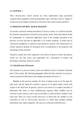
50,000 hp. Induction ac motors are characterized by a rotor which is neither a PM
nor a dc excited electromagnet. Instead current induced in a coil wound on the
rotor generates the interacting magnetic field of the rotor. This current is induced
from the stator coils. Figure 7.31 illustrates the basic concept. You can see that the ac
field of the stator produces a changing magnetic field passing through the closed
loop of the rotor. Faraday's law teaches us that [his changing flux will induce current
in the loop. This in turn creates a magnetic field in the rotor coil, which interacts
with the field of the stator. The bottom line is that a torque exists on the rotor
caused by these two fields.
Single-phase induction motors are used for applications of relatively low
power, say lessthan5hp(<3.7kW). Such motors are typical of those found in household
appliances, for example. For higher power we use three-phase ac excitation. Such
motors are available up to 10,000 hp.
In a control environment we want to have control over the speed of these
motors. The induction motor speed is dependent upon the ac excitation frequency,
much like Equation (7.6) for the synchronous motor, but with some small difference
referred to as the slip (in
FIGURE 7.31
The induction motor depends on a rotor field from current induced by ac field
coils, as shown in Figure 7.30.

32. FIGURE 7.32
ac motor control with a variable amplitude, variable frequency circuit using power
electronics, %)- Thus, speed control of both types can be affected by a variable
frequency ac excitaticm- In order to provide this we turn to power electronics.
Figure 7.32 provides a typical scbet where the three-phase ac (at 60 Hz) is rectified to
produce a variable amplitude dc w' by using SCRs with variable firing angle from the
control circuit. This voltage b f and then applied to a IGBT-based inverter whose
purpose is to produce a variable freqac voltage. The diodes across each IGBT provide
for current flow in reverse of the I Of course the sequence and speed of switching
provided by the control circuit di the frequency. The circuit could equally well use
GTOs, MOSFETs, or even BJT <Stepping Motor The stepping motor has increased
in importance in w because of the ease with which it can be interfaced with digital
circuits. A siepy.' •-a rotating machine thai actually completes a full rotation by
sequencing throws - discrete rotational steps. Each step position is an equilibrium
position in thai-excitation, the rotor position will stay at the latest step. Thus,
continuous roiatKc . by the input of a train of pulses, each of which causes an
advance of one step- k ontinuous rotation, but discrete, stepwise rotation. The
rotational rate is dem" —number of steps per revolution and the rate at which the
pulses are applied. A I is necessary to convert the pulse train into proper driving
signals for the mo—
EXAMPLE A stepper motor has 10° per step and must rotate at 250 rpm. What input
7.6 per second, is required?
Solution
A full revolution has 360°, so with 10° per step it will take 36 steps loco—lution.
Thus,
' rev V pulses i
250 —— 36 -—— = 9000 pulses/min

33. ^ mm / rev /
Therefore,
(9000 pulses/min )(lmin/60 s) = ISOpulses/s
FINAL CONTROL | 365
The operation of a stepping motor can be understood from the simple model
shown in Figure 7.33, which has 90° per step. In this motor, the rotor is a PM that is
driven by a particular set of electromagnets. In the position shown, the system is in
equilibrium and no motion occurs. The switches are typically solid-state devices, such
as transistors, SCRs, or TRIACs. The switch sequencer will direct the switches
through a sequence of positions as the pulses are received. The next pulse in Figure
7.33 will change S2 from C to D, resulting in the poles of that electromagnet reversing
fields.
Now, because the pole north/south orientation is different, the rotor is repelled
and attracted so that it moves to Ihe new position of equilibrium shown in Figure
7.34b. With the next pulse, Sl is changed to B, causing the same kind of pole reversal
and rotation of the PM to a new position, as shown in Figure 7.34c. Finally, the next
pulse causes S2 to switch to C again, and the PM rotor again steps lo a new
equilibrium position, as in Figure 7.34d- The next pulse will send the system back to
the original state and the rotor to the original position. This sequence is then repeated
as the pulse train comes in, resulting in a stepwise continuous rotation of the rotor PM.
Although this example illustrates the principle of operation, the most common stepper
motor does not use a PM,
FIGURE 7.33
An elementary stepping motor,

34. FIGURE 7.34
The four positions of the elementary stepper rotor.
FIGURE 7.35
Stepper with 8 rotor teeth and 12 stator poles. Note that the rotor teeth line up with the
A poles. With the next step, the rotor teeth will line up with the B poles, but rather a
rotor of magnetic material (not a magnet) with a certain numbc- -r This rotor is
driven by a phased arrangement of coils with a different numbe: :* so that the rotor
can never be in perfect alignment with the staler. Figure 7.35 • this for a rotor with 8
"teeth" and a stator with 12 "poles." One sel of fo« aligned, but the other four are
not. If excitation is placed on the next set of pota taken off the first set (A), then the
rotor will step once to come into alignmot
FINAL CONTROL | 367
B set of poles. The direction of rotation of stepper motors can be changed just by
changing the order in which different poles are activated and deactivated.
7.5.2 Pneumatic Actuators
The actuator often translates a control signal into a large force or torque as required
to manipulate some control element. The pneumatic actuator is most useful for such
translation.
The principle is based on the concept of pressure as force per unit area. If we imagine
that a net pressure difference is applied across a diaphragm of surface area A. then a
net force acts on the diaphragm given by
F=A(pf-pt) (7.7)
where pi — pz = pressure difference (Pa)
A = diaphragm area (m2)
F = force (N)

35. If we need to double the available force for a given pressure, it is merely necessary to
dou-ble the diaphragm area. Very large forces can be developed by standard signal-pressure
ranges of 3 to 15psi(20to lOOkPa). Many types of pneumatic actuators are
available, but perhaps the most common are those associated with control valves. We
will consider these in some detail to convey the general principles.
The action of a direct pneumatic actuator is shown in Figure 7.36. Figure 7.36
on the left shows the condition in the low signal-pressure state, where the spring, S,
main- tains the diaphragm and the connected control shaft in a position as shown. The
pres- sure on the opposite (spring) side of the diaphragm is maintained at atmospheric
pressure by the open hole, H. Increasing the control pressure (gauge pressure) applies
a force on Ihe diaphragm, forcing the diaphragm and connected shaft down against
the spring force. Figure 7,36 on the right shows this in the case of maximum control
pres sure and maximum travel of the shaft. The pressure and force are linearly
related, as shown in Equation (7.7), and the compression of a spring is linearly
related to forces. a8
FIGURE 7.36
A direct pneumatic actuator for converting pressure signals into mechanical shaft
motion.
368 CHAPTER 7
FIGURE 7.37
A reverse-acting pneumatic actuator.
discussed in Chapter 5, Then we see that the shaft position is linearly related to the ap-plied
control pressure
&.x = ^-Ap (7.8)

36. where A-t = shaft (ravel (m)
&p = applied gauge pressure (Pa)
A = diaphragm area (m2)
k = spring constant (N/m)
A reverse actuator, shown in Figure 7.37, moves the shaft in the opposite sense
frothe direct actuator but obeys the same operating principle. Thus, the shaft is pulled
in by (be application of a control pressure,
EXAMPLE Suppose a force of 400 N must be applied to open a valve. Find the
diaphragm area if a cc- 7.7 trol gauge pressure of 70 kPa (~ 10 psi) must provide
this force.
Solution
We must calculate the area from
F " A{p, - pt)
where our applied pressure is p; — p; because a gauge pressure is specified. Then
_F _ 400 N
p 7 X 104 Pa
A= 5.71 X lO^m2
or about 8,5 cm in diameter. The inherent compressibility of gases causes an upper
limit to the usefubeM ft f» for propagating force. Consider the pneumatic actuator of
Figure 7.36. When we ••an •"I tion to occur under low shaft load, we simply increase
pressure in the actuator vu i cr" lator. The regulator allows more gas from a high-pressure
reservoir to enter the se»»-

37. This increases the diaphragm force until it is able to move the shaft. Suppose the
shaft is connected to a very high load—that is, something icq^k very large force for
movement. In principle, it is simply a matter of increasing the fww
HNALCONTROL I 3—
of the input gas until the pressure X diaphragm area equals the required force- What
we find, however, is that as we try to raise the input gas pressure, large volumes of gas
must be passed into the actuator to bring about any pressure rise because the gas is
compressing; that is, its density is increasing.
7.5.3 Hydraulic Actuators
We have seen that there is an upper limit to the forces that can be applied using gas as
the working fluid. Yet there are many cases when large forces are required. In such
cases, a hy- draulic actuator may be employed. The basic principle is shown in Figure
7.38. The basic idea is the same as for pneumatic actuators, except that an
incompressible fluid is used to provide the pressure, which can be made very large by
adjusting the area of the forcing pis- ton, A]. The hydraulic pressure is given by
PH = Wi (7.9)
where py = hydraulic pressure (Pa)
F] = applied piston force (N)
A] = forcing piston area (m2)
This pressure is transferred equally throughout the liquid, so the resulting force on the
working piston is
m
(7.11)
^W = Pfi'^2

38. where FB, = force of working piston (N)
A; = working piston area (m3)
Thus, the working force is given in terms of the applied force by
a. Find the working force resulting from 200 N applied to a 1-cm-radius forcing
piston if the working piston has a radius of 6 cm.
b. Find the hydraulic pressure.
A, -4
FIGURE 7.38
A hydraulic actuator converts a small
force, Fi, into an amplified force, Fy,.
F, F»
Hydraulic flu id
374 | CHAPTER?
Reaction vassal
FIGURE 7.44
Control of heal into a reaction vessel through an electrical power amplifier.
7.6.3 Fluid Valves
The chemical and petroleum industries have many applications that require control
ctf fluid processes. Many other industries also depend in part on operations that
involve flu- ids and the regulation of fluid parameters. The word fluid here
represents either gasa liquids, or vapors. Many principles of control can be equally
applied to any of iheK

39. stales of matter, with only slight corrections. Many fluid operations require
regulan:*T of such quantities as density and composition, but by far the most
important control :rameter is flow rate. A regulation of flow rate emerges as the
regulatory parameter :":r reaction rate, temperature, composition, or a host of
other fluid properties. We will C--PI. sider in some detail that process-control
element specifically associated with flow—BE control valve.
Control -Valve Principles Flow rate in process control is usually exprc&scc
volume per unit time. If a mass flow rate is desired, it can be calculated from the
panx^u- fluid density. If a given fluid is delivered through a pipe, then the volume
flow rate u
Q = Av (LX=
where Q = flow rate (m'/s)
A = pipe area (m2)
V SE flow velocity (m/s)
FINAL CONTROL | 375
EXAMPLE Alcohol is pumped through a pipe of 10-cm diameter at 2 m/s flow
velocity. Find the vol-
7.9 lime flow rate.
Solution
A pipe of 10-cm diameter has a cross-sectional area of
-irJ2^ MtlO-'m)2
4 4
A =7.85 X lO^m2

40. Thus, the flow rate is
Q = Av = (7.85 X lO-'m2^ m/s)
0 = 0.0157 mVs
The purpose of the control valve is to regulate the flow rate of fluids through
pipes in the system- This is accomplished by placing a variable-size restriction in the
flow path, as shown in Figure 7.45. You can see that as the stem and plug move up
and down, the size of the opening between the plug and me seat changes, thus
changing (he flow rate. Note the direction of flow with respect to the seat and plug. If
the flow were reversed, force from the flow would tend to close the valve further at
small openings.
There will be a drop in pressure across such a restriction, and the flow rate varies
with the square root of this pressure drop, with an appropriate constant of
proportional- ity, shown by
(7.13)
fi== KV^p
where K = proportionality constant (mVs/Pa^2)
Ap = pi - P] == pressure difference (Pa)
Flow
SMU
FIGURE 7.45
A basic control-valve cross-section. The direction of flow is important for proper
valve
action.

41. EXAMPLE A pressure difference of 1.1 psi occurs across a constriction in a 5-cm-diameter
pipe. The 7.10 constriction constant is 0.009 mVs per kPa1''3. Find (a)
the flow rate in mVs and (b) the flow velocity in m/s.
Solution
First we note that 1.1 psi gives
Ap = (1.1 psi)(6.895 kPa/psi)
Ap = 7.5845 kPa
a. The flow rate is 'tT
Q = KV^p = (0.009)(7.5845)1/2
Q = 0.025 mVs
b. The flow velocity is found from
Q= Av
=0.= ,|" 0-025 mVs "I
v A L^(5X lO-^J
v = 12.7 m/s
The constant. K, depends on the size of the valve, the geometrical structure of re
delivery system, and. to some extent, on the material flowing through [he valve.
Nouactual pressure of the entire fluid delivery (and sink) system in which the valve is
u(and, hence, the flow rate) is not a predictable function of the valve opening only.
Bui -n- cause the valve opening does change flow rate, it provides a mechanism of
flow COBC"
Control -Valve Types The different types of control valves are classified by ——

42. lationship between the valve stem position and the flow rate through the valve-ftB"
control-valve characteristic is assigned with the assumptions that the stem
position B: cates the extent of the valve opening and that the pressure difference is
determined h" -• valve alone. Correction factors allow one to account for pressure
differences introd——b the whole system. Figure 7.46 shows a typical control valve
using a pneumatic aco—— tached to drive the stem and hence open and close the
valve. There are three basic nyc control valves, whose relationship between stem
position (as a percentage of full nape .J flow rate (as a percentage of maximum) is
shown in Figure 7.47.
The types are determined by the shape of the plug and seat, as shown in Fi| As
the stem and plug move with respect to the seat, the shape of the plug amount of
actual opening of the valve. 1. Quick Opening This type of valve is used
predominantly for full control applications. The valve characteristic of Figure 7.47
show's tively small motion of the valve stem results in maximum possfllie through
the valve. Such a valve, for example, may allow 90% of I rate with only a 30% travel
of the stem.
FINAL CONTROL | 377
FIGURE 7.46
A pneumatic actuator connected to a control valve- The actuator is driven by a current
through an 1/P converter.
Flow
Vtlve body
FIGURE 7.47
Three types of control vatves open differently as a function of valve stem position,
0.2 0.4 0.6 0.8 I

43. Sam petition 1 S/S,,,
2. Linear This type of vaive. as shown in Figure 7.47, has a flow rate that varies
linearly with the stem position. II represenis the ideal situation where the valve atone
determines the pressure drop. The relationship is expressed as
where Q = flow rate (m'/s)
Qmw = maximum flow rate (mVs)
S = stem position (m)
'max
maximum stem position (m)
3®B fl CHAPTER 7
1R
3. Equal Percentage A very important type of valve employed in flow con- trol has
a characteristic such that a given percentage change in stem position produces an
equivalent change in flow—that is, an equal percentage. Generally, this type of valve
does not shut off the flow completely in ils limit of stem travel. Thus, Q^ represents
the minimum flow when the stem is at one limit of its travel. At the other extreme,
the valve allows a flow Qmux as its maximum, open-valve flow rate. For this type,
we define rangeability, R, as the ratio
The curve in Figure 7.47 shows a typical equal percentage curve that depends on the
rangeability for its exact form. The curve shows that increase in flou. rate for a given
change in valve opening depends on the extent to which the valve is already open.
This curve is typically exponential in form and is rep- resented by where all terms
have been defined previously.

44. EXAMPLE An equal percentage valve has a maximum flow of 50 cmVs and a
minimum of 2 c 7.11 If the full travel is 3 cm, find the flow at a l-cm opening.
Solution
The rangeability is ^ = Qmu/Qmim
R = (50 cmVs}/(2 cmVs) = 25
Then the flow at a l-cm opening is
Q-Q^R5''--
Q= (2cmVs)(25)l"n/3nn
Q = 5.85 cmVs
Control -Valve Sizing Another important factor associated with all co valves
involves corrections to Equation (7.13) because of the nonideal character of the
materials that flow- A standard nomenclature is used to account for these colions,
depending on the liquid, gas, or steam nature of the fluid. These correction fallow
selection of the proper size of valve to accommodate the rate of flow that ihel tern
must support. The correction factor most commonly used at present is measian the
number of U.S. gallons of water per minute that flow through a fully open valve ia
pressure differential of 1 Ib per square inch. The correction factor is called the flow
coefficient and is designated as Cy. Using this factor, a liquid flow rate ia L" S Ions
per minute is