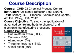
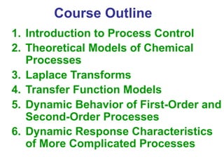
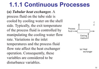
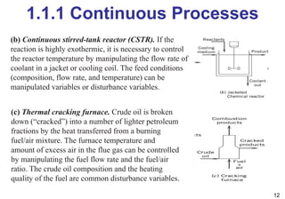
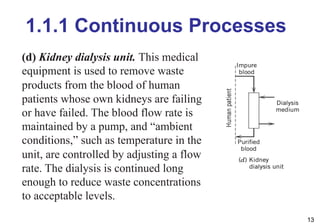
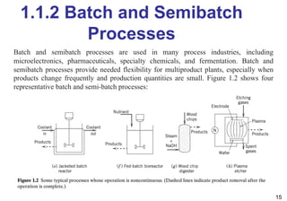
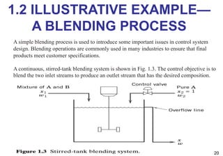
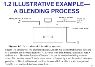
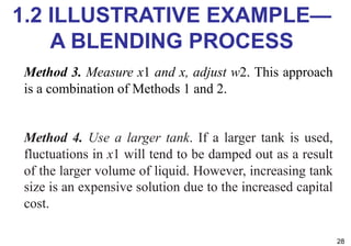
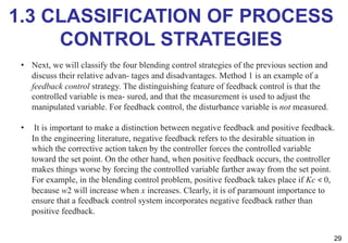
This document provides an overview of a chemical process control course. It includes: - A list of course policies including exams, assignments, and grading. - An outline of topics to be covered in the course ranging from process modeling to controller design. - An introduction to process control concepts including different types of processes (continuous, batch, semibatch), control variables, and strategies for controlling processes like a blending operation. The document provides details on the structure, content, and objectives of the chemical process control course.

1. 1
CHE403
Chemical Process
Control
Assistant Professor
Betül Gürünlü, PhD
Fall, 2023

2. 2
Course Description
Course: CHE403 Chemical Process Control
Instructor: Assistant Professor Betül Gürünlü
Text: Seborg, D.E., Process Dynamics and Control,
4th Ed., Wiley, USA, 2017.
Course Objective: To study the application of
advanced control methods to chemical and
electronic manufacturing processes
Course Policies:
• One midterm exam (30%),
• Quizzes (10%),
• Attendance (5%),
• Three homeworks (15%),
• A final exam (40%)

3. Course Outline
1. Introduction to Process Control
2. Theoretical Models of Chemical
Processes
3. Laplace Transforms
4. Transfer Function Models
5. Dynamic Behavior of First-Order and
Second-Order Processes
6. Dynamic Response Characteristics
of More Complicated Processes

4. Course Outline - Continued
7. Development of Empirical Models
from Process Data
8. Midterm Exam
9. Feedback Controllers
10. Control System Instrumentation
& Process Safety and Process
Control
11. Dynamic Behavior and Stability
of Closed-Loop Control Systems

5. Course Outline - Continued
12. PID Controller Design, Tuning,
and Troubleshooting & Control
Strategies at the Process Unit Level
13. Frequency Response Analysis
and Control System Design
14. Feedforward and Ratio Control
15. Final Exam

6. Introduction to Process Control
1. 1.1 Representative Process Control Problems
1.1.1.1 Continuous Processes
2.1.1.2 Batch and Semibatch Processes
2. 1.2 Illustrative Example—A Blending Process
3. 1.3 Classification of Process Control Strategies
1.3.1 Process Control Diagrams
4. 1.4 A More Complicated Example—A Distillation
Column
5. 1.5 The Hierarchy of Process Control Activities
6. 1.6 An Overview of Control System Design
Summary 6

7. Introduction to Process Control
• In recent years the performance requirements for process plants have become
increasingly difficult to satisfy. Stronger competition, tougher environmental
and safety regulations, and rapidly changing economic conditions have been
key factors. Consequently, product quality specifications have been tightened
and increased emphasis has been placed on more profitable plant operation. A
further complication is that modern plants have become more difficult to
operate because of the trend toward complex and highly integrated processes.
Thus, it is difficult to prevent disturbances from propagating from one unit to
other interconnected units.
• In view of the increased emphasis placed on safe, efficient plant operation, it
is only natural that the subject of process control has become increasingly
important in recent years. Without computer-based process control systems, it
would be impossible to operate modern plants safely and profitably while
satisfying product quality and environmental requirements. Thus, it is
important for chemical engineers to have an understanding of both the theory
and practice of process control.
7

8. Introduction to Process Control
• The two main subjects of this course are process dynamics and process control. The
term process dynamics refers to unsteady-state (or transient) process behavior. By
contrast, most of the chemical engineering curricula emphasize steady-state and
equilibrium conditions in such courses as material and energy balances,
thermodynamics, and transport phenomena. But the topic of process dynamics is also
very important. Transient operation occurs during important situations such as start-ups
and shutdowns, unusual process disturbances, and planned transitions from one
product grade to another. Consequently, the first part of this course is concerned with
process dynamics.
• The primary objective of process control is to maintain a process at the desired
operating conditions, safely and economically, while satisfying environmental and
product quality requirements. The subject of process control is concerned with how to
achieve these goals. In large-scale, integrated processing plants such as oil refineries or
ethylene plants, thousands of process variables such as compositions, temperatures,
and pressures are measured and must be controlled. Fortunately, thousands of process
variables (mainly flow rates) can usually be manipulated for this purpose. Feed-back
control systems compare measurements with their desired values and then adjust the
manipulated variables accordingly.
8

9. Introduction to Process Control
• Feedback control is a fundamental concept that is absolutely critical for both
biological and manmade systems. Without feedback control, it would be very
difficult, if not impossible, to keep complicated systems at the desired conditions.
Feedback control is embedded in many modern devices that we take for granted:
computers, cell phones, consumer electronics, air con- ditioning, automobiles,
airplanes, as well as automatic control systems for industrial processes. The scope and
history of feedback control and automatic control systems have been well described
elsewhere (Mayr, 1970; Åström and Murray, 2008; Blevins and Nixon, 2011).
• For living organisms, feedback control is essential to achieve a stable balance of
physiological variables, a condition that is referred to as homeostasis. In fact,
homeostasis is considered to be a defining feature of physiology (Widmaier et al.,
2011). In biology, feedback control occurs at many different levels including gene,
cellular, metabolic pathways, organs, and even entire ecosystems. For the human
body, feedback is essential to regulate critical physiological variables (e.g., tem-
perature, blood pressure, and glucose concentration) and processes (e.g., blood
circulation, respiration, and digestion). Feedback is also an important concept in
education and the social sciences, especially economics (Rao, 2013) and psychology
(Carver and Scheier, 1998).
9

10. 1.1 REPRESENTATIVE PROCESS
CONTROL PROBLEMS
• The foundation of process control is process understanding.
Thus, we begin this section with a basic question: what is a
process? For our purposes, a brief definition is appropriate:
• Process: The conversion of feed materials to products using
chemical and physical operations. In practice, the term
process tends to be used for both the processing operation
and the processing equipment.
• There are three broad categories of processes: contin- uous,
batch, and semibatch. Next, we consider repre- sentative
processes and briefly summarize key control issues.
10

11. 1.1.1 Continuous Processes
11
(a) Tubular heat exchanger. A
process fluid on the tube side is
cooled by cooling water on the shell
side. Typically, the exit temperature
of the process fluid is controlled by
manipulating the cooling water flow
rate. Variations in the inlet
temperatures and the process fluid
flow rate affect the heat exchanger
operation. Consequently, these
variables are considered to be
disturbance variables.

12. 1.1.1 Continuous Processes
12
(b) Continuous stirred-tank reactor (CSTR). If the
reaction is highly exothermic, it is necessary to control
the reactor temperature by manipulating the flow rate of
coolant in a jacket or cooling coil. The feed conditions
(composition, flow rate, and temperature) can be
manipulated variables or disturbance variables.
(c) Thermal cracking furnace. Crude oil is broken
down (“cracked”) into a number of lighter petroleum
fractions by the heat transferred from a burning
fuel/air mixture. The furnace temperature and
amount of excess air in the flue gas can be controlled
by manipulating the fuel flow rate and the fuel/air
ratio. The crude oil composition and the heating
quality of the fuel are common disturbance variables.

13. 1.1.1 Continuous Processes
13
(d) Kidney dialysis unit. This medical
equipment is used to remove waste
products from the blood of human
patients whose own kidneys are failing
or have failed. The blood flow rate is
maintained by a pump, and “ambient
conditions,” such as temperature in the
unit, are controlled by adjusting a flow
rate. The dialysis is continued long
enough to reduce waste concentrations
to acceptable levels.

14. 1.1.1 Continuous Processes
14
• Controlled variables (CVs): The process variables that are controlled. The
desired value of a controlled variable is referred to as its set point.
• Manipulated variables (MVs): The process variables that can be adjusted in
order to keep the controlled variables at or near their set points. Typically, the
manipulated variables are flow rates.
• Disturbance variables (DVs): Process variables that affect the controlled
variables but cannot be manipulated. Disturbances generally are related to changes
in the operating environment of the process: for example, its feed conditions or
ambient temperature. Some disturbance variables can be measured on-line, but
many cannot such as the crude oil composition for Process (c), a thermal cracking
furnace.
The specification of CVs, MVs, and DVs is a critical step in developing a control system.
The selections should be based on process knowledge, experience, and control objectives.
For each of these four examples, the process control problem has been characterized by
identifying three important types of process variables.

15. 1.1.2 Batch and Semibatch
Processes
15
Batch and semibatch processes are used in many process industries, including
microelectronics, pharmaceuticals, specialty chemicals, and fermentation. Batch and
semibatch processes provide needed flexibility for multiproduct plants, especially when
products change frequently and production quantities are small. Figure 1.2 shows four
representative batch and semi-batch processes:

16. 1.1.2 Batch and Semibatch
Processes
16
(e) Jacketed batch reactor. In a batch reactor, an initial
charge (e.g., reactants and catalyst) is placed in the
reactor, agitated, and brought to the desired starting
conditions. For exothermic reac- tions, cooling jackets
are used to keep the reactor temperature at or near the
desired set point. Typically, the reactor temperature is
regulated by adjusting the coolant flow rate. The endpoint
composition of the batch can be controlled by adjusting
the temperature set point and/or the cycle time, the time
period for reactor operation. At the end of the batch, the
reactor contents are removed and either stored or
transferred to another process unit such as a separation
process.

17. 1.1.2 Batch and Semibatch
Processes
17
(f) Semibatch bioreactor. For a semibatch reactor, one of
the two alternative operations is used: (i) a reactant is
gradually added as the batch proceeds or (ii) a product
stream is withdrawn during the reaction. The first
configuration can be used to reduce the side reactions
while the second configuration allows the reaction equilib-
rium to be changed by withdrawing one of the products
(Fogler, 2010).
For bioreactors, the first type of semibatch operation is
referred to as a fed-batch operation; it is shown in Fig.
1.2(f). In order to better reg- ulate the growth of the desired
microorganisms, a nutrient is slowly added in a
predetermined manner.

18. 1.1.2 Batch and Semibatch
Processes
18
(g) Semibatch digester in a pulp mill. Both
contin- uous and semibatch digesters are
used in paper manufacturing to break down
wood chips in order to extract the cellulosic
fibers. The end point of the chemical
reaction is indicated by the kappa number, a
measure of lignin content. It is controlled to
a desired value by adjust- ing the digester
temperature, pressure, and/or cycle time.

19. 1.1.2 Batch and Semibatch
Processes
19
(h) Plasma etcher in semiconductor processing. A
single wafer containing hundreds of printed circuits is
subjected to a mixture of etching gases under conditions
suitable to establish and main- tain a plasma (a high
voltage applied at high temperature and extremely low
pressure). The unwanted material on a layer of a
microelec- tronics circuit is selectively removed by
chemical reactions. The temperature, pressure, and flow
rates of etching gases to the reactor are controlled by
adjusting electrical heaters and control valves.

20. 1.2 ILLUSTRATIVE EXAMPLE—
A BLENDING PROCESS
20
A simple blending process is used to introduce some important issues in control system
design. Blending operations are commonly used in many industries to ensure that final
products meet customer specifications.
A continuous, stirred-tank blending system is shown in Fig. 1.3. The control objective is to
blend the two inlet streams to produce an outlet stream that has the desired composition.

21. 1.2 ILLUSTRATIVE EXAMPLE—
A BLENDING PROCESS
21
Stream 1 is a mixture of two chemical species, A and B. We assume that its mass flow rate
w1 is constant, but the mass fraction of A, x1, varies with time. Stream 2 consists of pure A
and thus x2 = 1. The mass flow rate of Stream 2, w2, can be manipulated using a control
valve. The mass fraction of A in the outlet stream is denoted by x and the desired value (set
point) by xsp. Thus for this control problem, the controlled variable is x, the manipulated
variable is w2, and the disturbance variable is x1.

22. 1.2 ILLUSTRATIVE EXAMPLE—
A BLENDING PROCESS
22
Next we consider two questions.
Design Question. If the nominal value of x1 is x1, what nominal flow rate
w2 is required to produce the desired outlet concentration, xsp?

23. 1.2 ILLUSTRATIVE EXAMPLE—
A BLENDING PROCESS
23
Equation 1-3 is the design equation for the blending system. If our assumptions are
correct and if x1 = ̅
𝑥1, then this value of w2 will produce the desired result, x = xsp. But
what happens if conditions change?
The overbar over a symbol denotes its nominal steady- state value, for example,
the value used in the process design. According to the process description, 𝑥! = 1
and ̅
𝑥 = xsp. Solving Eq. 1-1 for #
𝑤, substituting these values into Eq. 1-2, and
rearranging gives

24. 1.2 ILLUSTRATIVE EXAMPLE—
A BLENDING PROCESS
24
Control Question. Suppose that inlet concentration x1
varies with time. How can we ensure that the outlet
composition x remains at or near its desired value,
xsp ?
As a specific example, assume that x1 increases to a constant
value that is larger than its nominal value, ̅
𝑥1. It is clear that
the outlet composition will also increase due to the increase in
inlet composition. Consequently, at this new steady state, x >
xsp.

25. 1.2 ILLUSTRATIVE EXAMPLE—
A BLENDING PROCESS
25
Next we consider several strategies for reducing the effects of x1 disturbances on x.
Method 1. Measure x and adjust w2. It is reasonable to measure controlled variable x and then
adjust w2 accordingly. For example, if x is too high, w2 should be reduced; if x is too low, w2
should be increased. This control strategy could be implemented by a person (manual control).
However, it would normally be more convenient and economical to automate this simple task
(automatic control).
Method 1 can be implemented as a simple control algorithm (or control law),
where Kc is a constant called the controller gain. The symbols, w2(t) and x(t), indicate that w2
and x change with time. Equation 1-4 is an example of proportional control, because the
change in the flow rate, w2(t) − #
𝑤2, is proportional to the deviation from the set point, xsp –
x(t). Consequently, a large deviation from set point produces a large corrective action, while a
small deviation results in a small corrective action. Note that we require Kc to be positive
because w2 must increase when x decreases, and vice versa.

26. 1.2 ILLUSTRATIVE EXAMPLE—
A BLENDING PROCESS
26
A schematic diagram of Method 1 is shown in Fig. 1.4. The outlet concentration is
measured and transmitted to the controller as an electrical signal. (Electrical signals are
shown as dashed lines in Fig. 1.4.) The controller exe- cutes the control law and sends
an appropriate electrical signal to the control valve. The control valve opens or closes
accordingly.

27. 1.2 ILLUSTRATIVE EXAMPLE—
A BLENDING PROCESS
27
Method 2. Measure x1 , adjust w2. As an alternative to Method 1, we could measure
disturbance variable x1 and adjust w2 accordingly. Thus, if x1 > ̅
𝑥1, we would decrease
w2 so that w2 < #
𝑤2. If x1 < ̅
𝑥1, we would increase w2. A control law based on Method 2
can be obtained from Eq. 1-3 by replacing ̅
𝑥1 with x1(t) and #
𝑤2 with w2(t):
The schematic diagram for Method 2 is shown
in Fig. 1.5. Because Eq. 1-3 is valid only for
steady-state conditions, it is not clear just how
effective Method 2 will be during the transient
conditions that occur after an x1 disturbance.

28. 1.2 ILLUSTRATIVE EXAMPLE—
A BLENDING PROCESS
28
Method 3. Measure x1 and x, adjust w2. This approach
is a combination of Methods 1 and 2.
Method 4. Use a larger tank. If a larger tank is used,
fluctuations in x1 will tend to be damped out as a result
of the larger volume of liquid. However, increasing tank
size is an expensive solution due to the increased capital
cost.

29. 1.3 CLASSIFICATION OF PROCESS
CONTROL STRATEGIES
29
• Next, we will classify the four blending control strategies of the previous section and
discuss their relative advan- tages and disadvantages. Method 1 is an example of a
feedback control strategy. The distinguishing feature of feedback control is that the
controlled variable is mea- sured, and that the measurement is used to adjust the
manipulated variable. For feedback control, the disturbance variable is not measured.
• It is important to make a distinction between negative feedback and positive feedback.
In the engineering literature, negative feedback refers to the desirable situation in
which the corrective action taken by the controller forces the controlled variable
toward the set point. On the other hand, when positive feedback occurs, the controller
makes things worse by forcing the controlled variable farther away from the set point.
For example, in the blending control problem, positive feedback takes place if Kc < 0,
because w2 will increase when x increases. Clearly, it is of paramount importance to
ensure that a feedback control system incorporates negative feedback rather than
positive feedback.

30. 30