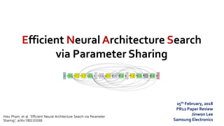
Efficient Neural Architecture Search
via Parameter Sharing
25th February, 2018
PR12 Paper Review
Jinwon Lee
Samsung Electronics
Hieu Pham, et al. “Efficient Neural Architecture Search via Parameter
Sharing”, arXiv:1802.03268
Reference Papers
• Barret Zoph, et al. “Neural Architecture Search with Reinforcement
Learning”, In ICLR, 2017
• Irwan Bello, et al. “Neural Optimizer Search with Reinforcement
Learning”, In ICML, 2017
• Barret Zoph, et al. “LearningTransferable Architectures for Scalable
Image Recognition”, In CVPR, 2018
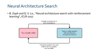
NeuralArchitecture Search
• B. Zoph and Q.V. Le., “Neural architecture search with reinforcement
learning”, ICLR-2017
Tesorflow Pre-trained Models
• https://github.com/tensorflow/models/tree/master/research/slim
NeuralArchitecture Search
• How controller RNN samples a simple convolutional network
Method
• Overall architectures of the convolutional nets are manually
predetermined
 Normal Cell – convolutional cells that return a feature map of the same
dimension
 Reduction Cell – convolutional cells that return a feature map where the
feature map height and width is reduced by a factor of two
• Using common heuristic to double the number of filters in the output
whenever the spatial activation size is reduced
Scalable Architectures for Image Classification
Models and Algorithms
Search Space in a Cell (Step 3 and 4)
Best Architecture (NASNet-A)
…5번
…5번
<Normal Cell>
<Reduction Cell>
NASNet-B
NASNet-C
Motivation
• NAS used 800 GPUs for 28days and NASNet used 450 GPUs for 3-4
days (i.e. 32,400-43,200 GPU hours)
• Meanwhile, using less resources tends to produce less compelling
results
• Computational bottleneck of NAS is the training of each child model
to convergence, only to measure its accuracy whilst throwing away
all the trained weights
Main Idea
Forcing all child models to share weights
to eschew training each child model from scratch to convergence
 Using Single GTX 1080Ti GPU, the search for architectures takes less
than 16 hours (compared to NAS, reduction is more than 1000x)
Directed Acyclic Graph(DAG)
• ENAS’s DAG is the superposition of all possible child models in a search
space of NAS, where the nodes represent the local computations and the
edges represent the flow of information.
• The local computations at each node have their own parameters, which
are used only when the particular computation is activated.
• Therefore, ENAS’s design allows parameters to be shared among all child
models
Directed Acyclic Graph(DAG)
• The graph represents the entire search space while the red arrows
define a model in the search space, which is decided by a controller.
• Here, node 1 is the input to the model whereas nodes 3 and 6 are the
model’s outputs.
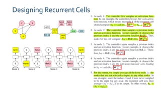
Designing RecurrentCells
Search Space for Recurrent Cells
• 4 activation functions are allowed
 tanh, ReLU, identity, sigmoid
• If the recurrent cell has N nodes,
 The search space has 4N x N! configuration
 When N = 12, there are approximately 1015 models in the search space
Training ENAS
• The controller network is an LSTM with 100 hidden units
• This LSTM samples decisions via softmax classifier, in an
autoregressive fashion
• In ENAS, there are two sets of learnable parameters
 The parameters of the controller LSTM, denoted by θ
 The shared parameters of child models, denoted by ω
• The first phase trains ω,
• The second phase trains θ
Deriving Architectures
• Sampling several models from the trained policy π(m, θ)
• Computing its reward on a single minibatch sampled from the
validation set
• The model with the highest reward is taken and retrained from
scratch
• training all the sampled models from scratch and selecting the model
with the highest performance is possible but it is not economical
Designing CNN
Search Spaces for CNN
• The 6 operations available for controller are
 Convolution with filter sizes 3x3 and 5x5
 Depthwise-separable convolutions with filter sizes 3x3 and 5x5
 Max pooling and average pooling of kernel size 3x3
• Making the described set of decisions for a total of L times,we can
sample a network of L layers.
• Since all decisions are independent, there are 6L × 2L(L−1)/2
• When L=12, resulting in 1.6 x 1029 possible networks
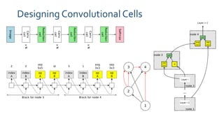
Designing Convolutional Cells
Search Spaces for Convolutional Cells
• The 5 available operations are
 Identity
 Separable convolution with kernel size 3x3 and 5x5
 Average pooling and max pooling with kernel size 3x3
• If there are B nodes, (5 x (B-2)!)4 cells are possible
• With B = 7, the search space can realize 1.3 x 10¹¹ final networks,
making it significantly smaller than the search space for entire
convolutional networks
Network Architecture for PennTreebank
Network Architecture for CIFAR-10(from macro
search space)
Network Architecture for CIFAR-10(from micro
search space)
Experimental Results
• Test perplexity on PennTreebank of ENAS and other baselines
Experimental Results
• Classification errors of ENAS and baselines on CIFAR-10

Efficient Neural Architecture Search via Parameter Sharing

  • 1.
    Efficient Neural ArchitectureSearch via Parameter Sharing 25th February, 2018 PR12 Paper Review Jinwon Lee Samsung Electronics Hieu Pham, et al. “Efficient Neural Architecture Search via Parameter Sharing”, arXiv:1802.03268
  • 2.
    Reference Papers • BarretZoph, et al. “Neural Architecture Search with Reinforcement Learning”, In ICLR, 2017 • Irwan Bello, et al. “Neural Optimizer Search with Reinforcement Learning”, In ICML, 2017 • Barret Zoph, et al. “LearningTransferable Architectures for Scalable Image Recognition”, In CVPR, 2018
  • 3.
    NeuralArchitecture Search • B.Zoph and Q.V. Le., “Neural architecture search with reinforcement learning”, ICLR-2017
  • 4.
    Tesorflow Pre-trained Models •https://github.com/tensorflow/models/tree/master/research/slim
  • 5.
    NeuralArchitecture Search • Howcontroller RNN samples a simple convolutional network
  • 6.
    Method • Overall architecturesof the convolutional nets are manually predetermined  Normal Cell – convolutional cells that return a feature map of the same dimension  Reduction Cell – convolutional cells that return a feature map where the feature map height and width is reduced by a factor of two • Using common heuristic to double the number of filters in the output whenever the spatial activation size is reduced
  • 7.
    Scalable Architectures forImage Classification
  • 8.
  • 9.
    Search Space ina Cell (Step 3 and 4)
  • 10.
  • 11.
  • 12.
  • 13.
  • 14.
    Motivation • NAS used800 GPUs for 28days and NASNet used 450 GPUs for 3-4 days (i.e. 32,400-43,200 GPU hours) • Meanwhile, using less resources tends to produce less compelling results • Computational bottleneck of NAS is the training of each child model to convergence, only to measure its accuracy whilst throwing away all the trained weights
  • 15.
    Main Idea Forcing allchild models to share weights to eschew training each child model from scratch to convergence  Using Single GTX 1080Ti GPU, the search for architectures takes less than 16 hours (compared to NAS, reduction is more than 1000x)
  • 16.
    Directed Acyclic Graph(DAG) •ENAS’s DAG is the superposition of all possible child models in a search space of NAS, where the nodes represent the local computations and the edges represent the flow of information. • The local computations at each node have their own parameters, which are used only when the particular computation is activated. • Therefore, ENAS’s design allows parameters to be shared among all child models
  • 17.
    Directed Acyclic Graph(DAG) •The graph represents the entire search space while the red arrows define a model in the search space, which is decided by a controller. • Here, node 1 is the input to the model whereas nodes 3 and 6 are the model’s outputs.
  • 18.
  • 19.
    Search Space forRecurrent Cells • 4 activation functions are allowed  tanh, ReLU, identity, sigmoid • If the recurrent cell has N nodes,  The search space has 4N x N! configuration  When N = 12, there are approximately 1015 models in the search space
  • 20.
    Training ENAS • Thecontroller network is an LSTM with 100 hidden units • This LSTM samples decisions via softmax classifier, in an autoregressive fashion • In ENAS, there are two sets of learnable parameters  The parameters of the controller LSTM, denoted by θ  The shared parameters of child models, denoted by ω • The first phase trains ω, • The second phase trains θ
  • 21.
    Deriving Architectures • Samplingseveral models from the trained policy π(m, θ) • Computing its reward on a single minibatch sampled from the validation set • The model with the highest reward is taken and retrained from scratch • training all the sampled models from scratch and selecting the model with the highest performance is possible but it is not economical
  • 22.
  • 23.
    Search Spaces forCNN • The 6 operations available for controller are  Convolution with filter sizes 3x3 and 5x5  Depthwise-separable convolutions with filter sizes 3x3 and 5x5  Max pooling and average pooling of kernel size 3x3 • Making the described set of decisions for a total of L times,we can sample a network of L layers. • Since all decisions are independent, there are 6L × 2L(L−1)/2 • When L=12, resulting in 1.6 x 1029 possible networks
  • 24.
  • 25.
    Search Spaces forConvolutional Cells • The 5 available operations are  Identity  Separable convolution with kernel size 3x3 and 5x5  Average pooling and max pooling with kernel size 3x3 • If there are B nodes, (5 x (B-2)!)4 cells are possible • With B = 7, the search space can realize 1.3 x 10¹¹ final networks, making it significantly smaller than the search space for entire convolutional networks
  • 26.
  • 27.
    Network Architecture forCIFAR-10(from macro search space)
  • 28.
    Network Architecture forCIFAR-10(from micro search space)
  • 29.
    Experimental Results • Testperplexity on PennTreebank of ENAS and other baselines
  • 30.
    Experimental Results • Classificationerrors of ENAS and baselines on CIFAR-10