SSD:
Single Shot MultiBox Detector
Wei Liu, et al., “SSD: Single Shot MultiBox Detector”, ECCV 2016
6th January, 2019
PR12 Paper Review
JinWon Lee
Samsung Electronics
Related Papers in PR12
• Faster R-CNN
 PR-013 : https://youtu.be/kcPAGIgBGRs
• YOLO
 PR-016 : https://youtu.be/eTDcoeqj1_w
• YOLO9000
 PR-023 : https://youtu.be/6fdclSGgeio
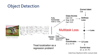
Object Detection
Slide from Stanford CS231n Lecture Slide
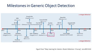
Milestones in Generic Object Detection
Figure from “Deep Learning for Generic Object Detection: A Survey”, arxiv1809.02165
2-stage detector
1-stage detector
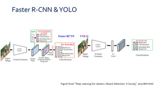
Faster R-CNN &YOLO
Figure from “Deep Learning for Generic Object Detection: A Survey”, arxiv1809.02165
Introduction
• Current state-of-the-art object detection systems are variants of the
following approach:
 Hypothesize bounding boxes, resample pixels or features for each box, and
apply a high-quality classifier.
• Computationally too intensive and too slow for real-time
applications.
 Faster R-CNN operates at only 7 FPS with mAP 73.2%
• Significantly increased speed comes only at the cost of significantly
decreased detection accuracy.
 YOLO operates at 45FPS with mAP 63.4%
Single Shot MultiBox Detector
• First deep network based object detector that does not resample
pixels or features for bounding box hypotheses(1-stage) and is as
accurate as approaches that do.
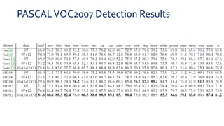
 59 FPS with mAP 74.3% onVOC2007 test
Model
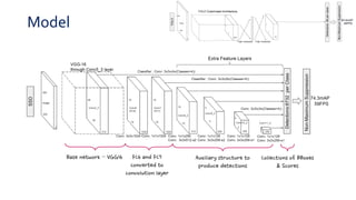
Base network – VGG16 FC6 and FC7
converted to
convolution layer
Auxiliary structure to
produce detections
Collections of BBoxes
& Scores
Multi-scale Feature Maps for Detection
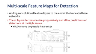
• Adding convolutional feature layers to the end of the truncated base
networks.
• These layers decrease in size progressively and allow predictions of
detections at multiple scales.
 YOLO use only single scale feature map.
Convolutional Predictors for Detection
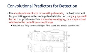
• For a feature layer of size m x n with p channels, the basic element
for predicting parameters of a potential detection is a 3 x 3 x p small
kernel that produces either a score for a category, or a shape offset
relative to the default box coordinates.
 YOLO has a fully connected layer for a score and a bbox coordinates.
Default Boxes and Aspect Ratios
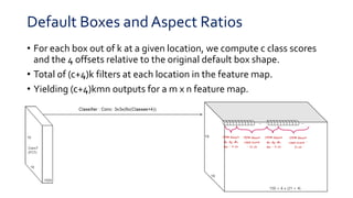
• For each box out of k at a given location, we compute c class scores
and the 4 offsets relative to the original default box shape.
• Total of (c+4)k filters at each location in the feature map.
• Yielding (c+4)kmn outputs for a m x n feature map.
......
19
19
1번째 bbox의
dx, dy, dh,
dw – 4 ch
1번째 bbox의
class score
– 21 ch
2번째 bbox의
dx, dy, dh,
dw – 4 ch
2번째 bbox의
class score –
21 ch
150 = 6 x (21 + 4)
Training – Matching Strategy
• Matching each ground truth box to the default box with the best
jaccard overlap. Every ground truth box has at least 1
correspondence.
• Then, matching default boxes to any ground truth with jaccard
overlap higher than a threshold(0.5).
Jaccard Overlap =
Figure from Wikipedia
Training Objective
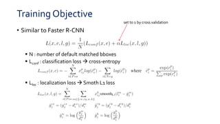
• Similar to Faster R-CNN
 N : number of default matched bboxes
 Lconf : classification loss  cross-entropy
 Lloc : localization loss  Smoth L1 loss
set to 1 by cross validation
Choosing Scales and Aspect Ratios for Default
Boxes
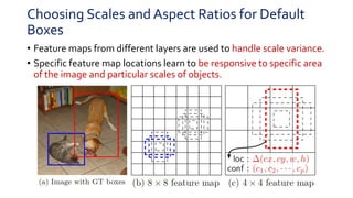
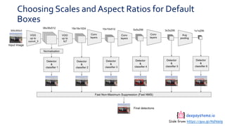
• Feature maps from different layers are used to handle scale variance.
• Specific feature map locations learn to be responsive to specific area
of the image and particular scales of objects.
Choosing Scales and Aspect Ratios for Default
Boxes
Slide from https://goo.gl/NsP6Wg
Choosing Scales and Aspect Ratios for Default
Boxes
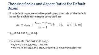
• If m default maps are used for prediction, the scale of the default
boxes for each feature map is computed as:
• smin is 0.2 and smax is 0.9
• For example (PASCALVOC 2007)
 sk is 0.1, 0.2, 0.375, 0.55, 0.725. 0.9
 means 30, 60, 112.5, 165, 217.5, 270 pixels @ input image(300x300)
Choosing Scales and Aspect Ratios for Default
Boxes
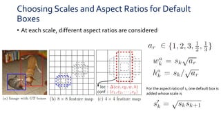
• At each scale, different aspect ratios are considered
For the aspect ratio of 1, one default box is
added whose scale is
Hard Negative Mining
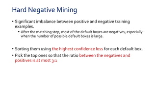
• Significant imbalance between positive and negative training
examples.
 After the matching step, most of the default boxes are negatives, especially
when the number of possible default boxes is large.
• Sorting them using the highest confidence loss for each default box.
• Pick the top ones so that the ratio between the negatives and
positives is at most 3:1
Data Augmentation
• Use the entire original input image.
• Sample a patch so that the minimum jaccard overlap with the
objects is 0.1, 0.3, 0.5, 0.7 or 0.9.
• Randomly sample a patch.
• The size of each sampled patch is [0,1, 1] of the original image size
• Aspect ratio is between ½ and 2.
• Horizontally flipped with probability of 0.5
Experimental Results
• Base Network
 VGG16 with fc6 and fc7 converted to conv layers and pool5 from 2x2 – s2 to
3x3 – s1 using atrous algorithm, removed fc8 and dropout
 Fine-tuned using SGD with momentum
PASCALVOC2007 Detection Results
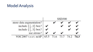
Model Analysis
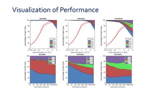
Visualization of Performance
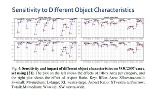
Sensitivity to Different Object Characteristics
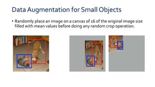
Data Augmentation for Small Objects
• Randomly place an image on a canvas of 16 of the original image size
filled with mean values before doing any random crop operation.
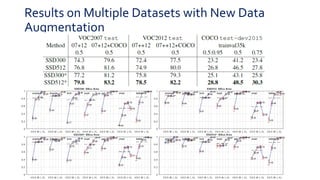
Results on Multiple Datasets with New Data
Augmentation
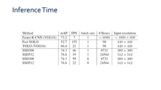
InferenceTime
Conclusions
• Single-shot object detector for multiple categories
• One key feature is multiple convolutional maps to deal with different
scales
• More default bounding boxes, the better results obtained
• Comparable accuracy to state-of-the-are object detectors but much
faster
Thank you

PR-132: SSD: Single Shot MultiBox Detector

  • 1.
    SSD: Single Shot MultiBoxDetector Wei Liu, et al., “SSD: Single Shot MultiBox Detector”, ECCV 2016 6th January, 2019 PR12 Paper Review JinWon Lee Samsung Electronics
  • 2.
    Related Papers inPR12 • Faster R-CNN  PR-013 : https://youtu.be/kcPAGIgBGRs • YOLO  PR-016 : https://youtu.be/eTDcoeqj1_w • YOLO9000  PR-023 : https://youtu.be/6fdclSGgeio
  • 3.
    Object Detection Slide fromStanford CS231n Lecture Slide
  • 4.
    Milestones in GenericObject Detection Figure from “Deep Learning for Generic Object Detection: A Survey”, arxiv1809.02165 2-stage detector 1-stage detector
  • 5.
    Faster R-CNN &YOLO Figurefrom “Deep Learning for Generic Object Detection: A Survey”, arxiv1809.02165
  • 6.
    Introduction • Current state-of-the-artobject detection systems are variants of the following approach:  Hypothesize bounding boxes, resample pixels or features for each box, and apply a high-quality classifier. • Computationally too intensive and too slow for real-time applications.  Faster R-CNN operates at only 7 FPS with mAP 73.2% • Significantly increased speed comes only at the cost of significantly decreased detection accuracy.  YOLO operates at 45FPS with mAP 63.4%
  • 7.
    Single Shot MultiBoxDetector • First deep network based object detector that does not resample pixels or features for bounding box hypotheses(1-stage) and is as accurate as approaches that do.  59 FPS with mAP 74.3% onVOC2007 test
  • 8.
    Model Base network –VGG16 FC6 and FC7 converted to convolution layer Auxiliary structure to produce detections Collections of BBoxes & Scores
  • 9.
    Multi-scale Feature Mapsfor Detection • Adding convolutional feature layers to the end of the truncated base networks. • These layers decrease in size progressively and allow predictions of detections at multiple scales.  YOLO use only single scale feature map.
  • 10.
    Convolutional Predictors forDetection • For a feature layer of size m x n with p channels, the basic element for predicting parameters of a potential detection is a 3 x 3 x p small kernel that produces either a score for a category, or a shape offset relative to the default box coordinates.  YOLO has a fully connected layer for a score and a bbox coordinates.
  • 11.
    Default Boxes andAspect Ratios • For each box out of k at a given location, we compute c class scores and the 4 offsets relative to the original default box shape. • Total of (c+4)k filters at each location in the feature map. • Yielding (c+4)kmn outputs for a m x n feature map. ...... 19 19 1번째 bbox의 dx, dy, dh, dw – 4 ch 1번째 bbox의 class score – 21 ch 2번째 bbox의 dx, dy, dh, dw – 4 ch 2번째 bbox의 class score – 21 ch 150 = 6 x (21 + 4)
  • 12.
    Training – MatchingStrategy • Matching each ground truth box to the default box with the best jaccard overlap. Every ground truth box has at least 1 correspondence. • Then, matching default boxes to any ground truth with jaccard overlap higher than a threshold(0.5). Jaccard Overlap = Figure from Wikipedia
  • 13.
    Training Objective • Similarto Faster R-CNN  N : number of default matched bboxes  Lconf : classification loss  cross-entropy  Lloc : localization loss  Smoth L1 loss set to 1 by cross validation
  • 14.
    Choosing Scales andAspect Ratios for Default Boxes • Feature maps from different layers are used to handle scale variance. • Specific feature map locations learn to be responsive to specific area of the image and particular scales of objects.
  • 15.
    Choosing Scales andAspect Ratios for Default Boxes Slide from https://goo.gl/NsP6Wg
  • 16.
    Choosing Scales andAspect Ratios for Default Boxes • If m default maps are used for prediction, the scale of the default boxes for each feature map is computed as: • smin is 0.2 and smax is 0.9 • For example (PASCALVOC 2007)  sk is 0.1, 0.2, 0.375, 0.55, 0.725. 0.9  means 30, 60, 112.5, 165, 217.5, 270 pixels @ input image(300x300)
  • 17.
    Choosing Scales andAspect Ratios for Default Boxes • At each scale, different aspect ratios are considered For the aspect ratio of 1, one default box is added whose scale is
  • 18.
    Hard Negative Mining •Significant imbalance between positive and negative training examples.  After the matching step, most of the default boxes are negatives, especially when the number of possible default boxes is large. • Sorting them using the highest confidence loss for each default box. • Pick the top ones so that the ratio between the negatives and positives is at most 3:1
  • 19.
    Data Augmentation • Usethe entire original input image. • Sample a patch so that the minimum jaccard overlap with the objects is 0.1, 0.3, 0.5, 0.7 or 0.9. • Randomly sample a patch. • The size of each sampled patch is [0,1, 1] of the original image size • Aspect ratio is between ½ and 2. • Horizontally flipped with probability of 0.5
  • 20.
    Experimental Results • BaseNetwork  VGG16 with fc6 and fc7 converted to conv layers and pool5 from 2x2 – s2 to 3x3 – s1 using atrous algorithm, removed fc8 and dropout  Fine-tuned using SGD with momentum
  • 21.
  • 22.
  • 23.
  • 24.
    Sensitivity to DifferentObject Characteristics
  • 25.
    Data Augmentation forSmall Objects • Randomly place an image on a canvas of 16 of the original image size filled with mean values before doing any random crop operation.
  • 26.
    Results on MultipleDatasets with New Data Augmentation
  • 27.
  • 28.
    Conclusions • Single-shot objectdetector for multiple categories • One key feature is multiple convolutional maps to deal with different scales • More default bounding boxes, the better results obtained • Comparable accuracy to state-of-the-are object detectors but much faster
  • 29.