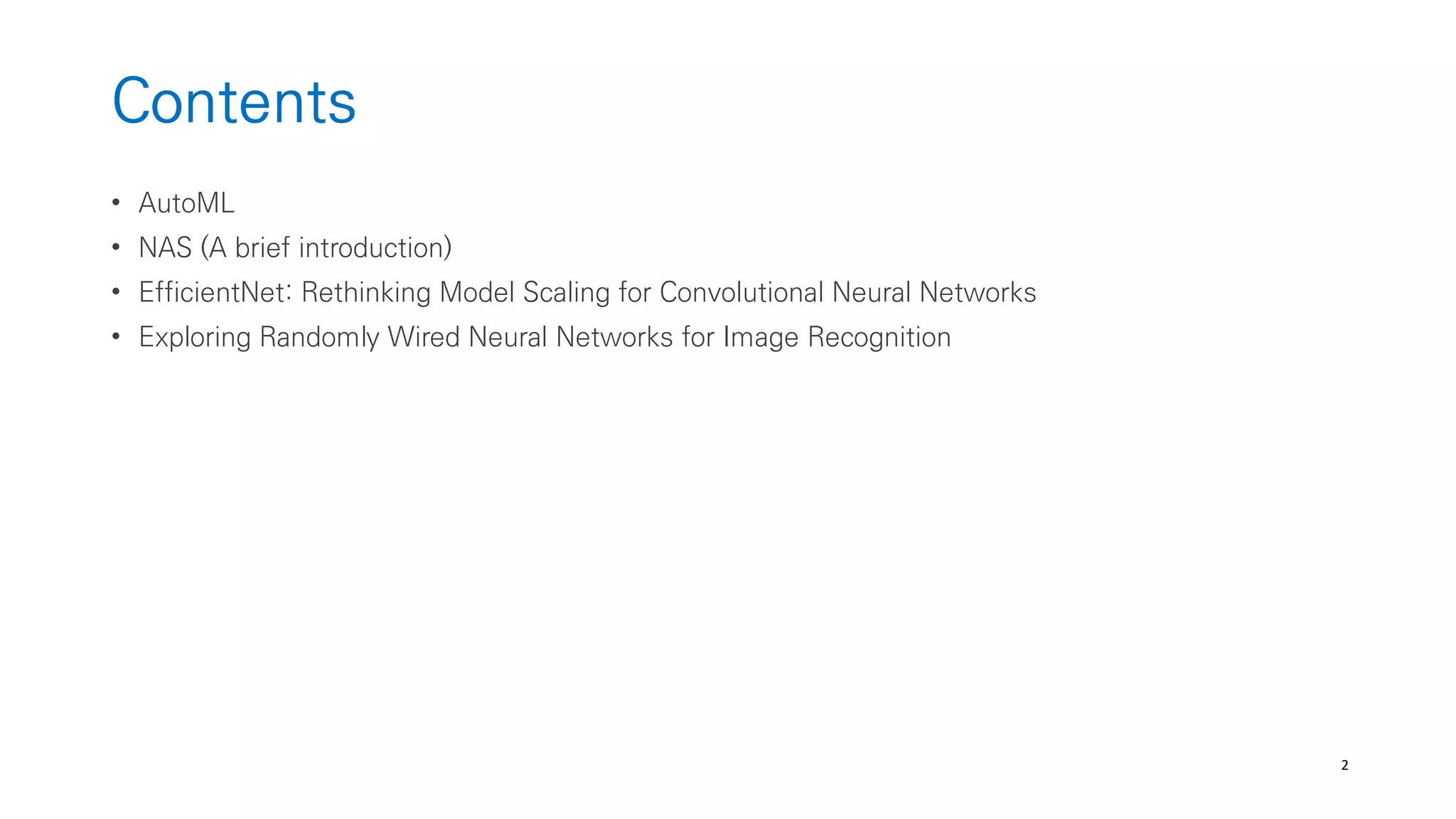
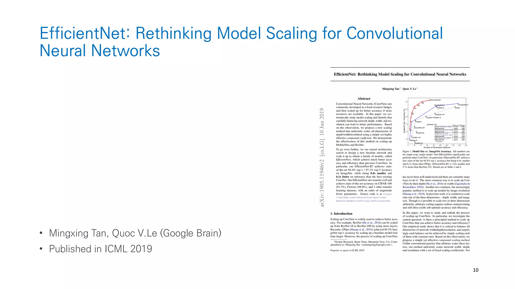
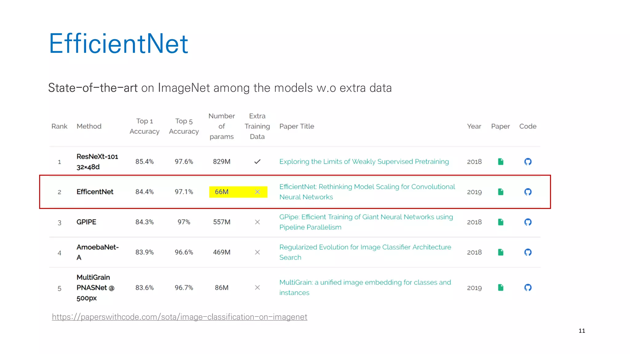
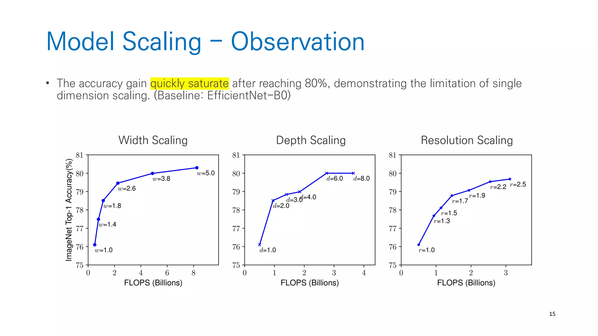
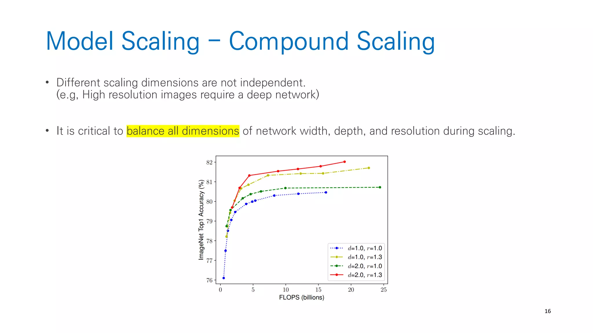
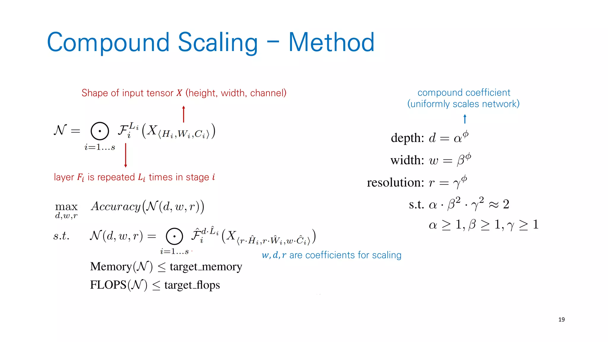
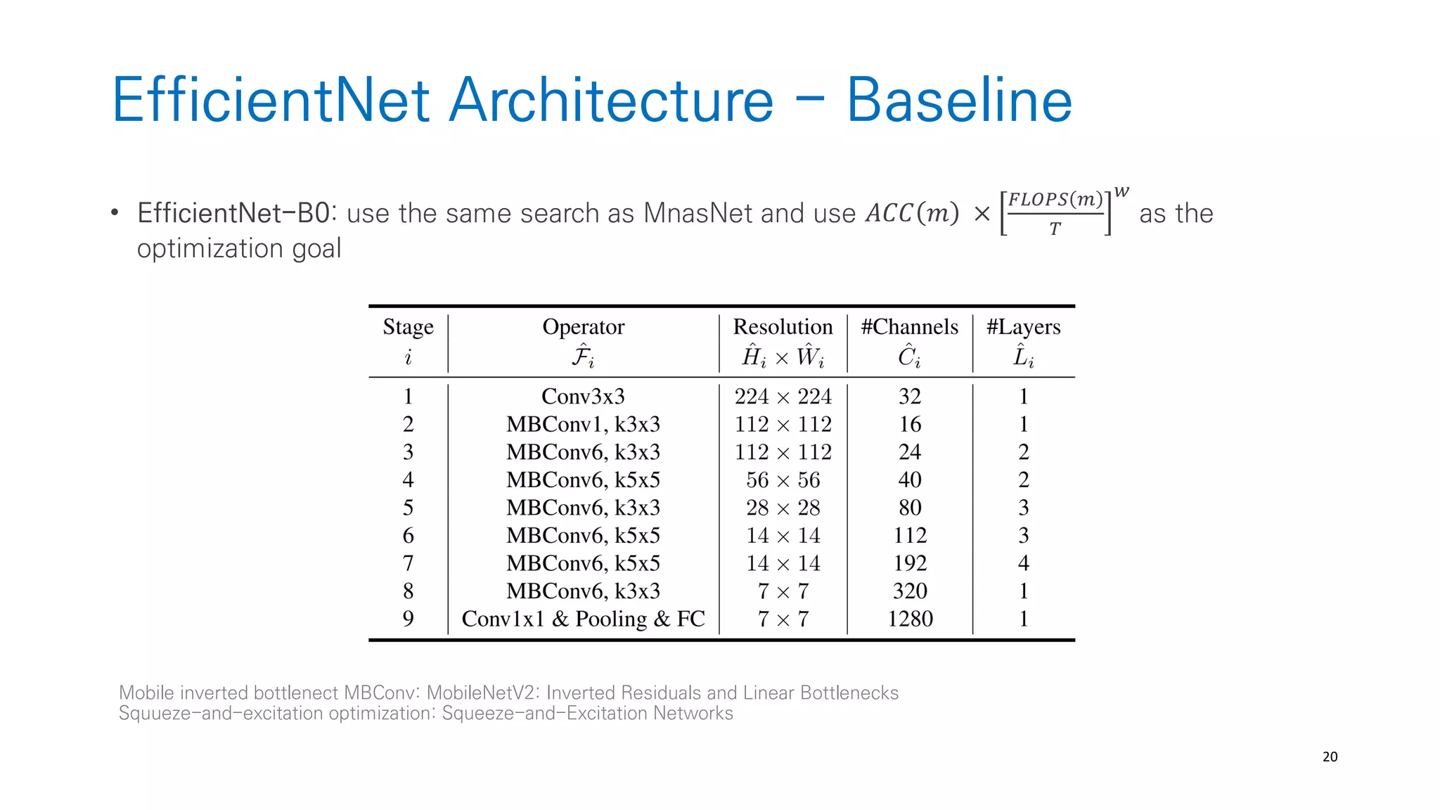
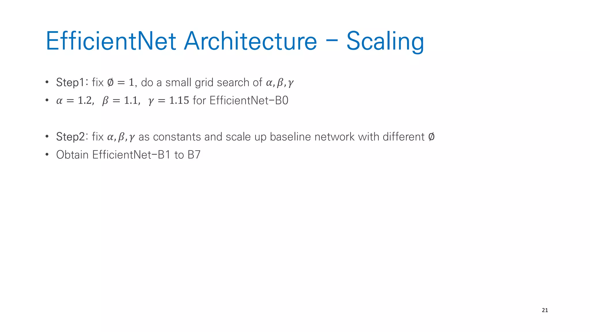
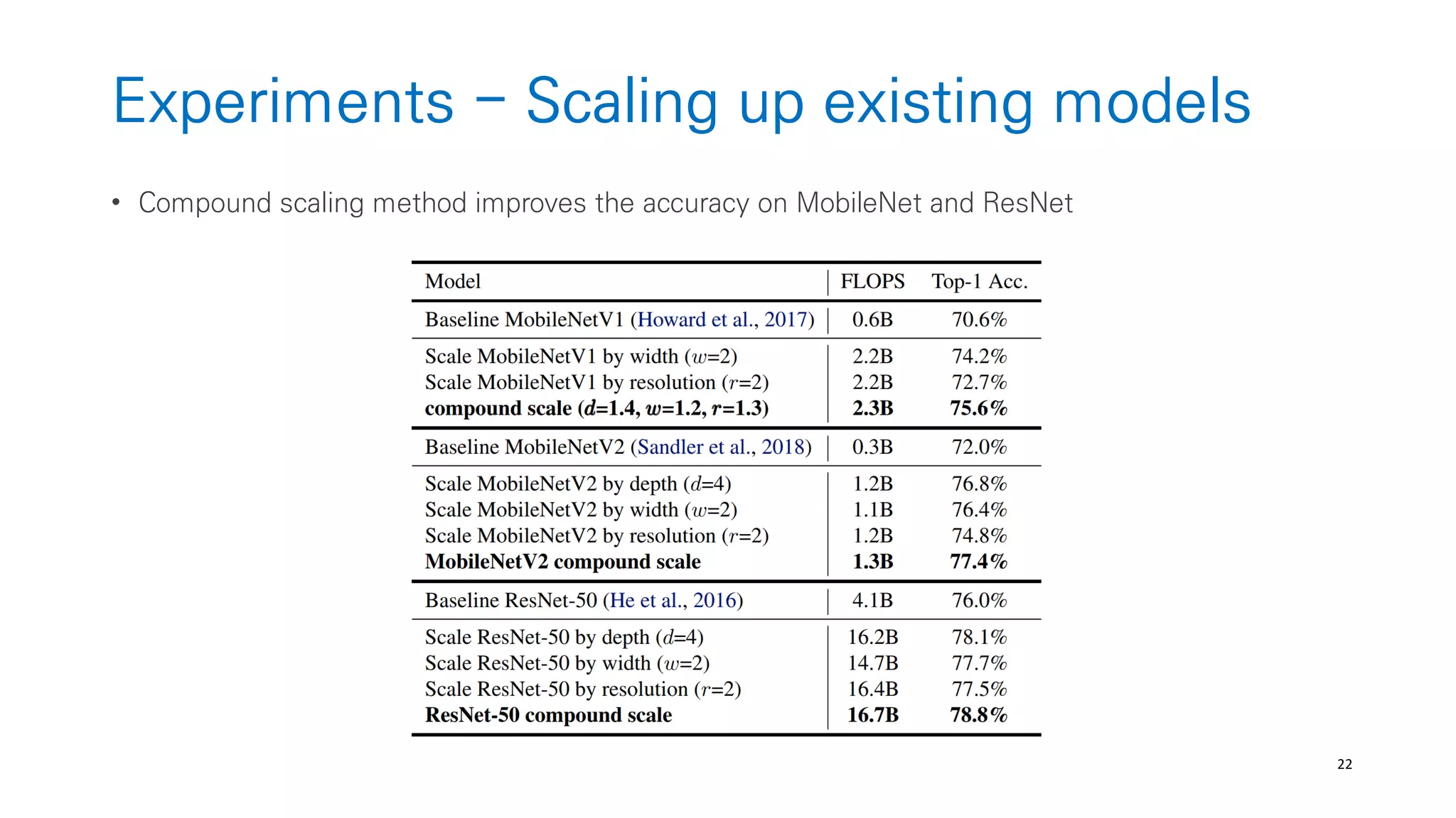
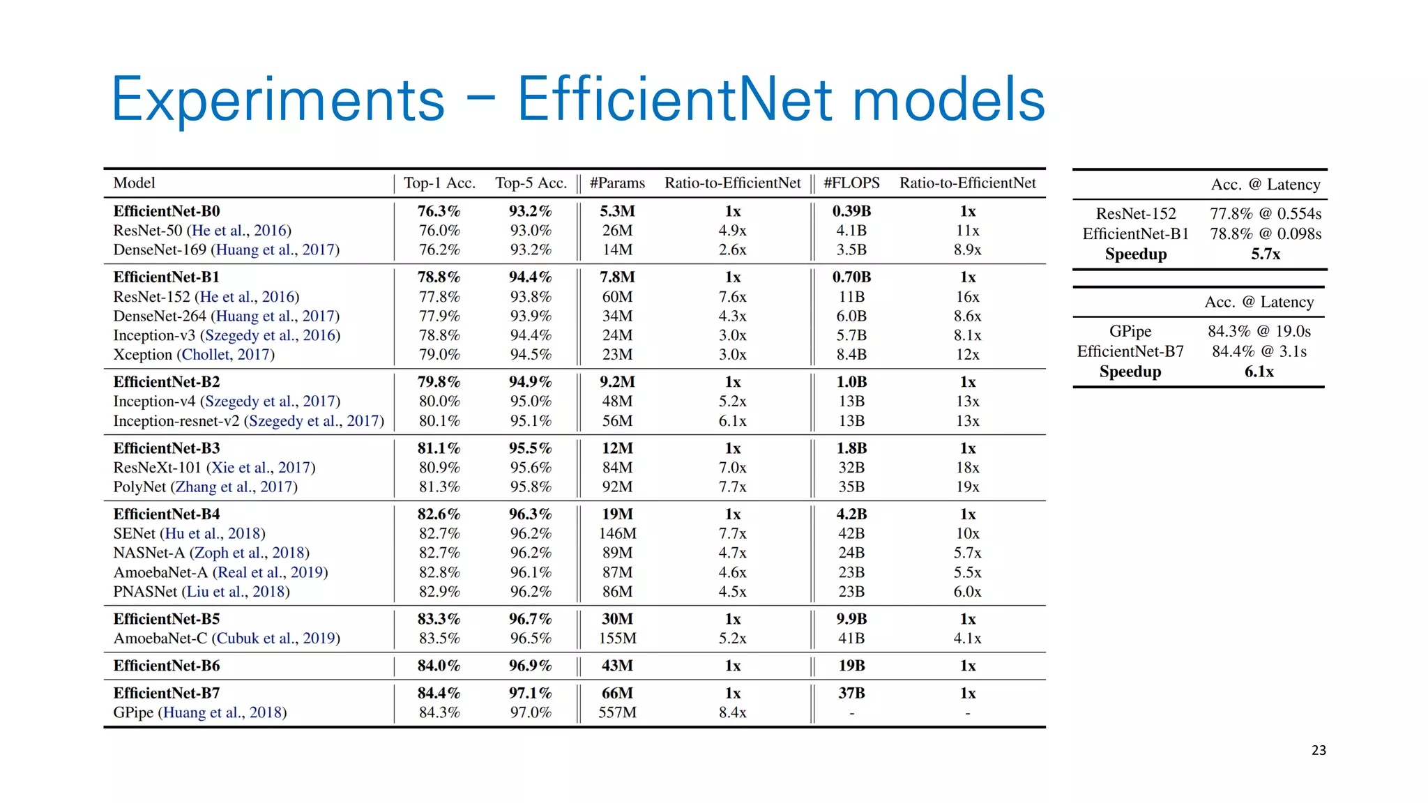
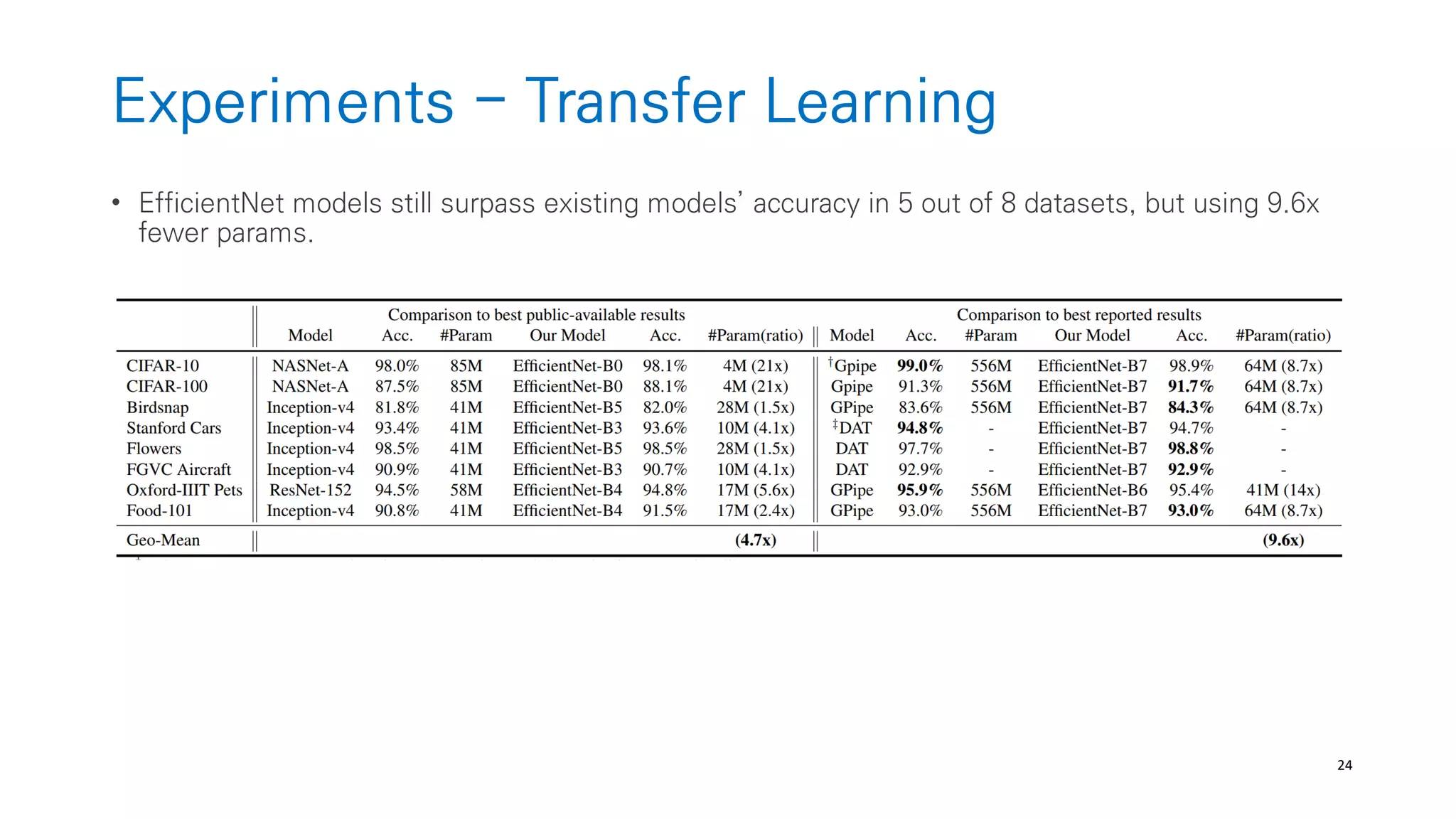
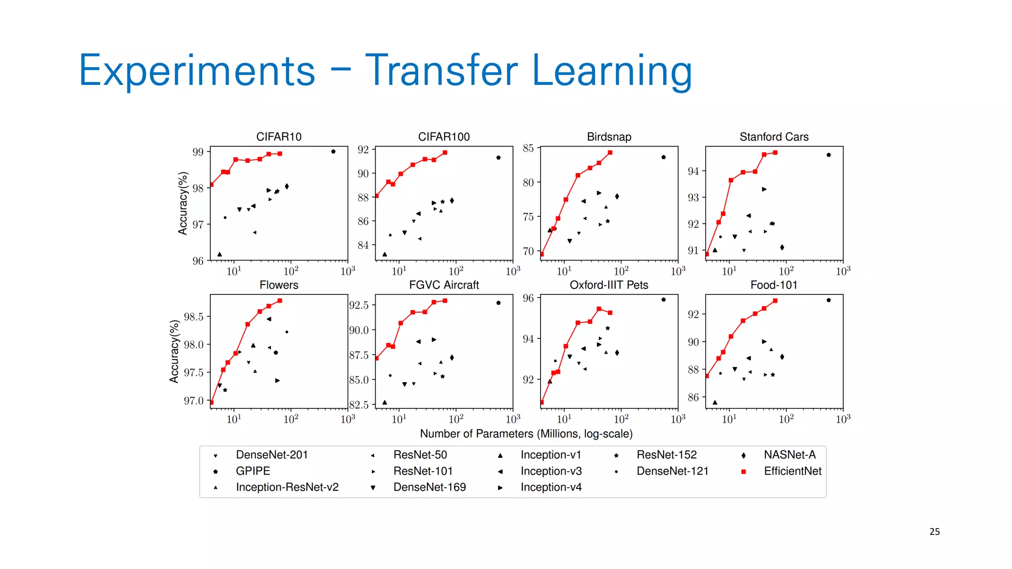
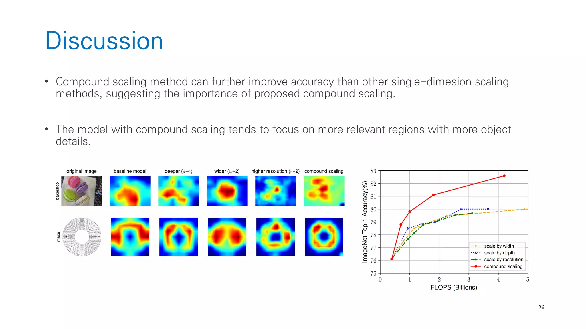
The document discusses AutoML and Neural Architecture Search (NAS), highlighting EfficientNet and randomly wired neural networks for image recognition. EfficientNet emphasizes compound scaling for improved accuracy with fewer parameters, while the research on randomly wired networks explores the potential for novel network designs that could enhance performance. Overall, the text underscores the significance of network generation methods in the evolution of neural architecture search.

1. 1
DaeJin Kim
2019.07
2019.07 - AutoML and
Neural Architecture Search
: EfficientNet, RandomWire

2. 2
Contents
• AutoML
• NAS (A brief introduction)
• EfficientNet: Rethinking Model Scaling for Convolutional Neural Networks
• Exploring Randomly Wired Neural Networks for Image Recognition

3. 3
AutoML
• Machine Learning for designing machine learning models
• Feature Engineering
• Deep Feature Synthesis
• One button machine
• R2n (Feature Learning From Relational Databases)
• Architecture Search
• NAS
• NasNet
• mNasNet
• DARTS
• Hyperparameter Optimization
• Auto-keras
• hyperopt

4. 4
NAS
• Neural Architecture Search with Reinforcement Learning
• Google Brain
• Published in ICLR 2017

5. 5
NAS
https://www.slideshare.net/KihoSuh/neural-architecture-search-with-reinforcement-learning-76883153

6. 6
Concept
• Select operation using RNN controller
• Train RNN controller using Reinforcement Learning

7. 7
Experiment - CNN
• Select # filtres, filter height/width, stride height/width using RNN controller
• For cifar-10 problem, it takes almost a month using 800 GPUs

8. 8
Experiment - RNN
• Select aggregation functions, and activation functions using RNN controller
• For penn treebank problem, it uses 160 CPUs
• Use tree structure referencing LSTM

9. 9
Experiment

10. 10
EfficientNet: Rethinking Model Scaling for Convolutional
Neural Networks
• Mingxing Tan, Quoc V.Le (Google Brain)
• Published in ICML 2019

11. 11
EfficientNet
State-of-the-art on ImageNet among the models w.o extra data
https://paperswithcode.com/sota/image-classification-on-imagenet

12. 12
Motivation
• “Although higher accuracy is critical for many applications,
we have already hit the hardware memory limit”
• Architecture Search for larger models requires much larger design space and much more
expensive tuning cost.
• How to do scaling without tedious manual tuning?

13. 13
Model Scaling - Dimensions
• Depth (# layers): Deeper ConvNet can capture richer and more complex features, and generalize
well on new tasks
• Width (# channels): Wider networks tend to be able to capture more find-grained features and are
easier to train / Difficulties in capturing higher level features
• Resolution (image sizes): ConvNets can potentially capture more fine-grained patterns

14. 14
Model Scaling - Dimensions

15. 15
Model Scaling - Observation
• The accuracy gain quickly saturate after reaching 80%, demonstrating the limitation of single
dimension scaling. (Baseline: EfficientNet-B0)
Width Scaling Depth Scaling Resolution Scaling

16. 16
Model Scaling - Compound Scaling
• Different scaling dimensions are not independent.
(e.g, High resolution images require a deep network)
• It is critical to balance all dimensions of network width, depth, and resolution during scaling.

17. 17
layer 𝐹𝑖 is repeated 𝐿𝑖 times in stage 𝑖
Shape of input tensor 𝑋 (height, width, channel)
Compound Scaling - Definition

18. 18
Compound Scaling - Problem
𝑤, 𝑑, 𝑟 are coefficients for scaling
layer 𝐹𝑖 is repeated 𝐿𝑖 times in stage 𝑖
Shape of input tensor 𝑋 (height, width, channel)

19. 19
Compound Scaling - Method
𝑤, 𝑑, 𝑟 are coefficients for scaling
layer 𝐹𝑖 is repeated 𝐿𝑖 times in stage 𝑖
Shape of input tensor 𝑋 (height, width, channel) compound coefficient
(uniformly scales network)

20. 20
EfficientNet Architecture - Baseline
• EfficientNet-B0: use the same search as MnasNet and use 𝐴𝐶𝐶 𝑚 ×
𝐹𝐿𝑂𝑃𝑆 𝑚
𝑇
𝑤
as the
optimization goal
Mobile inverted bottlenect MBConv: MobileNetV2: Inverted Residuals and Linear Bottlenecks
Squueze-and-excitation optimization: Squeeze-and-Excitation Networks

21. 21
EfficientNet Architecture - Scaling
• Step1: fix ∅ = 1, do a small grid search of 𝛼, 𝛽, 𝛾
• 𝛼 = 1.2, 𝛽 = 1.1, 𝛾 = 1.15 for EfficientNet-B0
• Step2: fix 𝛼, 𝛽, 𝛾 as constants and scale up baseline network with different ∅
• Obtain EfficientNet-B1 to B7

22. 22
Experiments - Scaling up existing models
• Compound scaling method improves the accuracy on MobileNet and ResNet

23. 23
Experiments - EfficientNet models

24. 24
Experiments - Transfer Learning
• EfficientNet models still surpass existing models’ accuracy in 5 out of 8 datasets, but using 9.6x
fewer params.

25. 25
Experiments - Transfer Learning

26. 26
Discussion
• Compound scaling method can further improve accuracy than other single-dimesion scaling
methods, suggesting the importance of proposed compound scaling.
• The model with compound scaling tends to focus on more relevant regions with more object
details.

27. 27
Exploring Randomly Wired Neural Networks for Image
Recognition
• Facebook AI Research (FAIR)
• 2019.04.02

28. 28
Exploring Randomly Wired Neural Networks for Image
Recognition
• Several random networks have competitive accuracy on the ImageNet benchmark

29. 29
Motivation
• How computational networks are wired is crucial for building intelligent machines.
(connectionist approach, e.g., ResNet, DenseNet…)
• NAS network generator is hand designed and the space of allowed wiring patterns is constrained
in a small subset of all possible graphs
• What happens if we lossen this constraint and design novel network generators?

30. 30
Network Generators
• Define a network generator as a mapping 𝑔 from a parameter space 𝜃 to a space of neural
network architectures 𝒩, 𝑔: 𝜃 ↦ 𝒩
• Generator 𝑔 determines how the computational graph is wired
• The parameters 𝜃 specify the instantiated network and many contain diverse information.
• Ex) ResNet
𝑔: produces a stack of blocks that compute 𝑥 + ℱ(𝑥)
𝜃: specify # stages, # residual blocks for each stages, depth/width/filter sizes, activation types…

31. 31
Stochastic Network Generators
• 𝑔 𝜃 performs a deterministic mapping
• Add a seed of a pseudo-random number 𝑠
• Stochastic network generators 𝑔(𝜃, 𝑠) can construct a (pseudo) random family of networks.

32. 32
NAS from the generator perspective
• The rules of the NAS generator:
• A cell always accepted the activations of the outputs nodes from the 2 immediately preceeding cells.
• Each cell contains 5 nodes that are wired to 2 and only 2 existing nodes
• All nodes that have no output in a cell are concatenated by an extra node to form a valid DAG for the cell.
• Network space 𝒩 has been carefully restricted by hand-designed rules
• The manual design in the NAS network generator is a strong prior, which represents a meta-
optimization beyond the search over 𝜃 (by RL), and 𝑠 (by random search)

33. 33
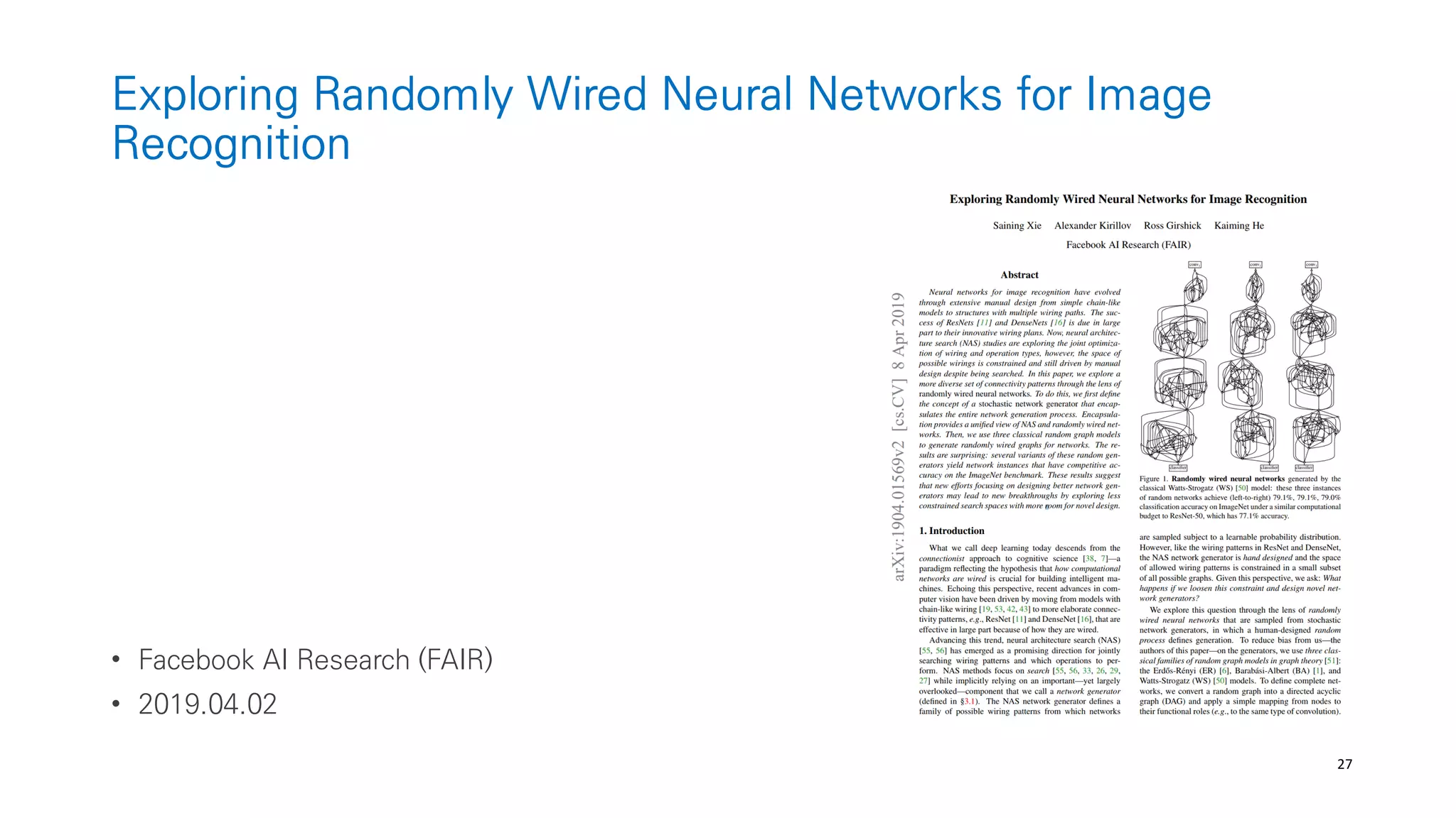
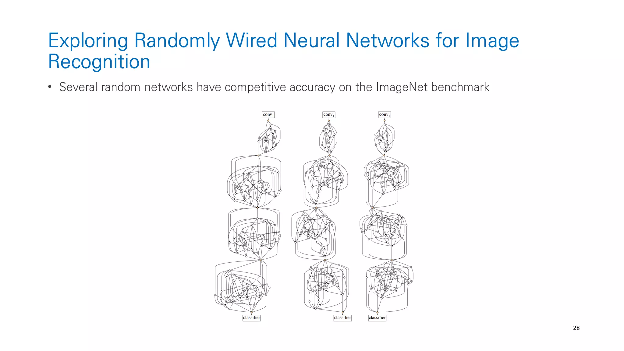
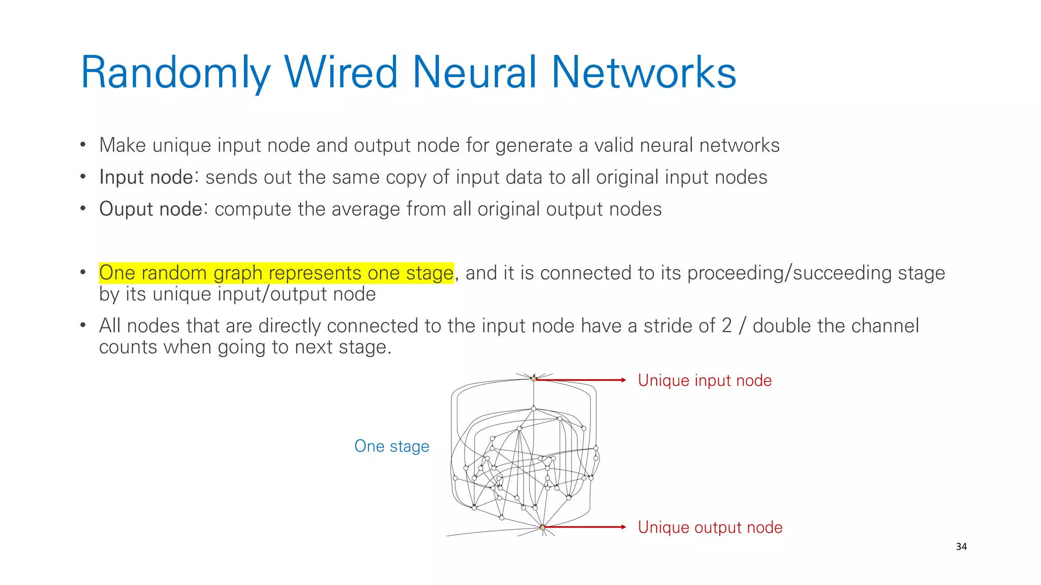
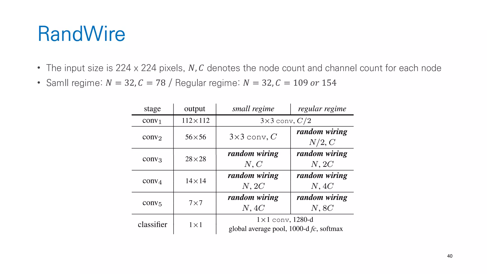
Randomly Wired Neural Networks
• Generate a general graphs w.o restricting how the graphs correspond to neural-networks
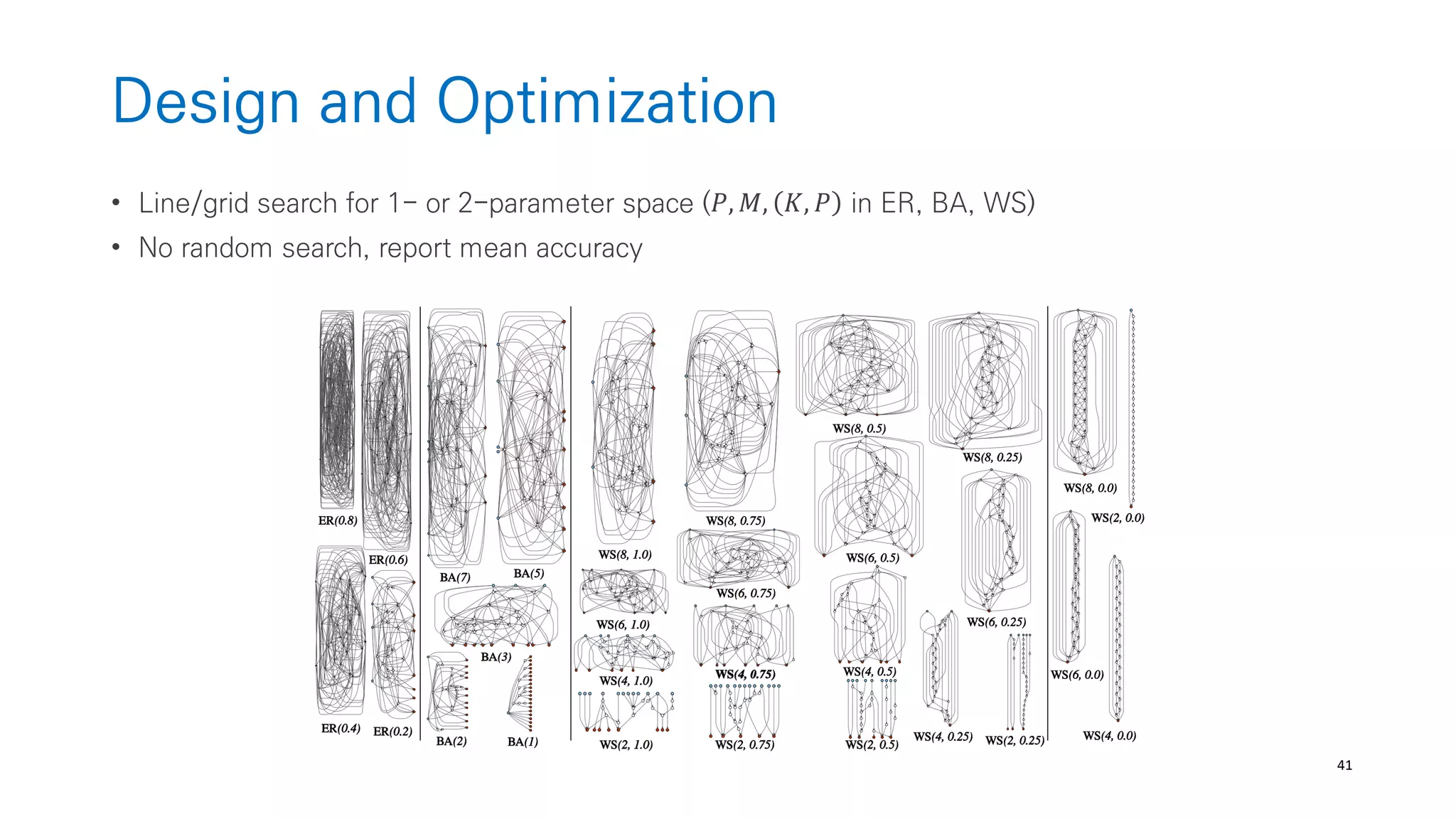
(from graph theory like ER, BA, WS)
• The edges are data flow (send data from one node to another node)
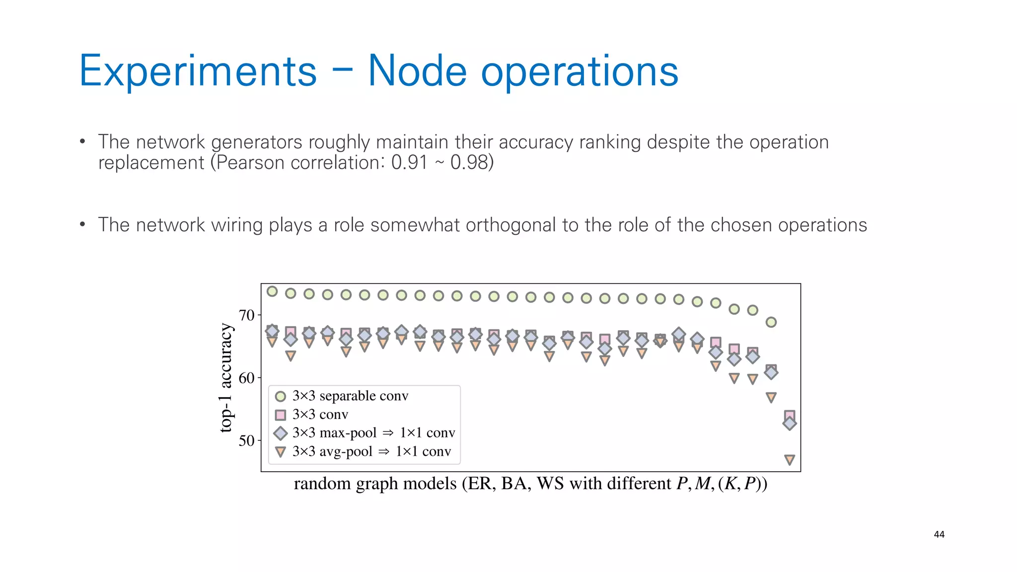
• Node operation
Aggregation: The input data are combied via a weighted sum; The weights are positive
Transformation: The aggregated data is processed by [ReLU-convolution-BN]
All nodes have same type of convolution!
Distribtuion: The same copy of the transformed data is sent out to other nodes.

34. 34
Randomly Wired Neural Networks
• Make unique input node and output node for generate a valid neural networks
• Input node: sends out the same copy of input data to all original input nodes
• Ouput node: compute the average from all original output nodes
• One random graph represents one stage, and it is connected to its proceeding/succeeding stage
by its unique input/output node
• All nodes that are directly connected to the input node have a stride of 2 / double the channel
counts when going to next stage.
Unique input node
Unique output node
One stage

35. 35
Operation Properties
• Maintains the same number of output channels as input channels
• Transformed data can be combined with the data from any other nodes
• FLOPS and params count of a graph are roughly proportional to the number of nodes
• Differences in task performance are therefore reflective of the properties of the wiring patterns

36. 36
Random Graph Models - Erdős–Rényi (ER)
• An edge between two nodes is connected with probability 𝑃, independent of all other nodes and
edges.
• Any graph with 𝑁 nodes has non-zero probability of being generated.
• A graph generated by ER(P) model has high probability of being a single connected component if
𝑃 >
ln 𝑁
𝑁
. It provides an implicit bias introduced by a generator.

37. 37
Random Graph Models - Barabási–Albert (BA)
• Generates a random graph by sequentially adding new nodes
• Initial state is 𝑀 nodes without any edges, sequentially adds a new node with 𝑀 new edges.
• Conncected to an existing node 𝑣 with probability proportional to 𝑣’s degree.
• Has exactly 𝑀 ∙ (𝑁 − 𝑀) edges (Subset of all possible 𝑁-node graphs)

38. 38
Random Graph Models - Watts–Strogatz (WS)
• Small-world graphs
• Initially, each node is connected to its 𝐾/2 neightbors on both sides (regular graph)
• In a clockwise loop, for every node 𝑣, the edge that connects 𝑣 to its clockwise 𝑖-th next node is
rewired with probability 𝑃
• Has exactly 𝑁 ∙ 𝐾 edges (Subset of all possible 𝑁-node graphs)

39. 39
Convert to DAGs
• Assign indcies to all nodes in a graph
• Set the direction of every edge as pointing from the smaller-index node to the larger-index one
• ER: indices are assigned in a random order
• BA: the initial 𝑀 nodes are assigned indices 1 to 𝑀, and all other nodes are indexed following their
order of adding to the graph
• WS: indices are assigned sequentially in the clockwise order

40. 40
RandWire
• The input size is 224 x 224 pixels, 𝑁, 𝐶 denotes the node count and channel count for each node
• Samll regime: 𝑁 = 32, 𝐶 = 78 / Regular regime: 𝑁 = 32, 𝐶 = 109 𝑜𝑟 154

41. 41
Design and Optimization
• Line/grid search for 1- or 2-parameter space (𝑃, 𝑀, 𝐾, 𝑃 in ER, BA, WS)
• No random search, report mean accuracy

42. 42
Experiments - Random graph generators
• All networks provide decent accuracy, and converge (None of them fails to converge)
• The variation among the random network instances is low
• Different random generators may have a gap between their mean accuracies.
• The random generator design plays an important role in the accuracy

43. 43
Experiments - Graph Damage
• Randomly removing one node or edge
• ER, BA, and WS behave differently under such damage

44. 44
Experiments - Node operations
• The network generators roughly maintain their accuracy ranking despite the operation
replacement (Pearson correlation: 0.91 ~ 0.98)
• The network wiring plays a role somewhat orthogonal to the role of the chosen operations

45. 45
Experiments - Comparisons (similar FLOPs)
• Small regime • Regular regime
• Larger regime

46. 46
Experiments - Transfer learning
• The features learned by randomly wired networks can also transfer

47. 47
Discussion
• Network generators are important to Neural Architecture Search (AutoML)
• New efforts focusing on designing better network generators may lead to new breakthroughs by
exploring less constrained search spaces with more room for novel design
• Our community have transitioned from designing features to designing a network that learns
features
• New transition from designing an individual network to designing a network generator may be
possible