This copyright notice specifies that DeepLearning.AI slides are distributed under a Creative Commons license, can be used non-commercially for education

1. Copyright Notice
These slides are distributed under the Creative Commons License.
DeepLearning.AI makes these slides available for educational purposes. You may not
use or distribute these slides for commercial purposes. You may make copies of these
slides and use or distribute them for educational purposes as long as you
cite DeepLearning.AI as the source of the slides.
For the rest of the details of the license, see
https://creativecommons.org/licenses/by-sa/2.0/legalcode

2. Neural Architecture Search
Welcome

3. Neural Architecture Search
Hyperparameter tuning

4. Neural Architecture Search
● Neural architecture search (NAS) is is a technique for automating the
design of artificial neural networks
● It helps finding the optimal architecture
● This is a search over a huge space
● AutoML is an algorithm to automate this search

5. Types of parameters in ML Models
● Trainable parameters:
○ Learned by the algorithm during training
○ e.g. weights of a neural network
● Hyperparameters:
○ set before launching the learning process
○ not updated in each training step
○ e.g: learning rate or the number of units in a dense layer

6. Manual hyperparameter tuning is not scalable
● Hyperparameters can be numerous even for small models
● e.g shallow DNN:
○ Architecture choices
○ activation functions
○ Weight initialization strategy
○ Optimization hyperparameters such as learning rate, stop condition
● Tuning them manually can be a real brain teaser
● Tuning helps with model performance

7. Automating hyperparameter tuning with Keras Tuner
● Automation is key: open source resources to the rescue
● Keras Tuner:
○ Hyperparameter tuning with Tensorflow 2.0.
○ Many methods available

8. Neural Architecture Search
Keras Autotuner Demo

9. Setting up libraries and dataset
import tensorflow as tf
from tensorflow import keras
mnist = tf.keras.datasets.mnist
(x_train, y_train),(x_test, y_test) = mnist.load_data()
x_train, x_test = x_train / 255.0, x_test / 255.0

10. Deep learning “Hello world!”
model = tf.keras.models.Sequential([
tf.keras.layers.Flatten(input_shape=(28, 28)),
tf.keras.layers.Dense(512, activation='relu'),
tf.keras.layers.Dropout(0.2),
tf.keras.layers.Dense(10, activation='softmax')
])
model.compile(optimizer='adam',
loss='sparse_categorical_crossentropy',
metrics=['accuracy'])
model.fit(x_train, y_train, epochs=5)
model.evaluate(x_test, y_test)

11. Model performance
Epoch 1/5
1875/1875 - 10s 5ms/step - loss: 0.3603 - accuracy: 0.8939
Epoch 2/5
1875/1875 - 10s 5ms/step - loss: 0.1001 - accuracy: 0.9695
Epoch 3/5
1875/1875 - 10s 5ms/step - loss: 0.0717 - accuracy: 0.9781
Epoch 4/5
1875/1875 - 10s 5ms/step - loss: 0.0515 - accuracy: 0.9841
Epoch 5/5
1875/1875 - 10s 5ms/step - loss: 0.0432 - accuracy: 0.9866

12. Parameters rational: if any
model = tf.keras.models.Sequential([
tf.keras.layers.Flatten(input_shape=(28, 28)),
tf.keras.layers.Dense(512, activation='relu'),
tf.keras.layers.Dropout(0.2),
tf.keras.layers.Dense(10, activation='softmax')
])
model.compile(optimizer='adam',
loss='sparse_categorical_crossentropy',
metrics=['accuracy'])
model.fit(x_train, y_train, epochs=5)
model.evaluate(x_test, y_test)

13. Is this architecture optimal?
● Do the model need more or less hidden units to perform well?
● How does model size affect the convergence speed?
● Is there any trade off between convergence speed, model size and
accuracy?
● Search automation is the natural path to take
● Keras tuner built in search functionality.

14. Automated search with Keras tuner
# First, install Keras Tuner
!pip install -q -U keras-tuner
# Import Keras Tuner after it has been installed
import kerastuner as kt

15. Building model with iterative search
def model_builder(hp):
model = keras.Sequential()
model.add(keras.layers.Flatten(input_shape=(28, 28)))
hp_units = hp.Int('units', min_value=16, max_value=512, step=16)
model.add(keras.layers.Dense(units=hp_units, activation='relu'))
model.add(tf.keras.layers.Dropout(0.2))
model.add(keras.layers.Dense(10))
model.compile(optimizer='adam',loss='sparse_categorical_crossentropy',
metrics=['accuracy'])
return model

16. Search strategy
tuner = kt.Hyperband(model_builder,
objective='val_accuracy',
max_epochs=10,
factor=3,
directory='my_dir',
project_name='intro_to_kt')
Other flavors: RandomSearch // BayesianOptimization // Sklearn

17. Callback configuration
stop_early =
tf.keras.callbacks.EarlyStopping(monitor='val_loss',
patience=5)
tuner.search(x_train,
y_train,
epochs=50,
validation_split=0.2,
callbacks=[stop_early])

18. Search output
Trial 24 Complete [00h 00m 22s]
val_accuracy: 0.3265833258628845
Best val_accuracy So Far: 0.5167499780654907
Total elapsed time: 00h 05m 05s
Search: Running Trial #25
Hyperparameter |Value |Best Value So Far
units |192 |48
tuner/epochs |10 |2
tuner/initial_e...|4 |0
tuner/bracket |1 |2
tuner/round |1 |0
tuner/trial_id |a2edc917bda476c...|None

19. Back to your model
model = tf.keras.models.Sequential([
tf.keras.layers.Flatten(input_shape=(28, 28)),
tf.keras.layers.Dense(48, activation='relu'),
tf.keras.layers.Dropout(0.2),
tf.keras.layers.Dense(10, activation='softmax')
])

20. Training output
Epoch 1/5
1875/1875 - 3s 1ms/step - loss: 0.6427 - accuracy: 0.8090
Epoch 2/5
1875/1875 - 3s 1ms/step - loss: 0.2330 - accuracy: 0.9324
Epoch 3/5
1875/1875 - 3s 1ms/step - loss: 0.1835 - accuracy: 0.9448
Epoch 4/5
1875/1875 - 3s 1ms/step - loss: 0.1565 - accuracy: 0.9515
Epoch 5/5
1875/1875 - 3s 1ms/step - loss: 0.1393 - accuracy: 0.9564

21. AutoML
Intro to AutoML

22. Outline
● Introduction to AutoML
● Neural Architecture Search
● Search Space and Search Strategies
● Performance Estimation
● AutoML on the Cloud

23. Automated Machine Learning (AutoML)
Auto ML
Data
Pipeline
Model
Training
Model
Deployment
Model
Monitoring
Discovery

24. Data
Validation
Feature
Engineering
Train Model
Data
Ingestion
Validate
Model
AutoML automates the entire ML workflow

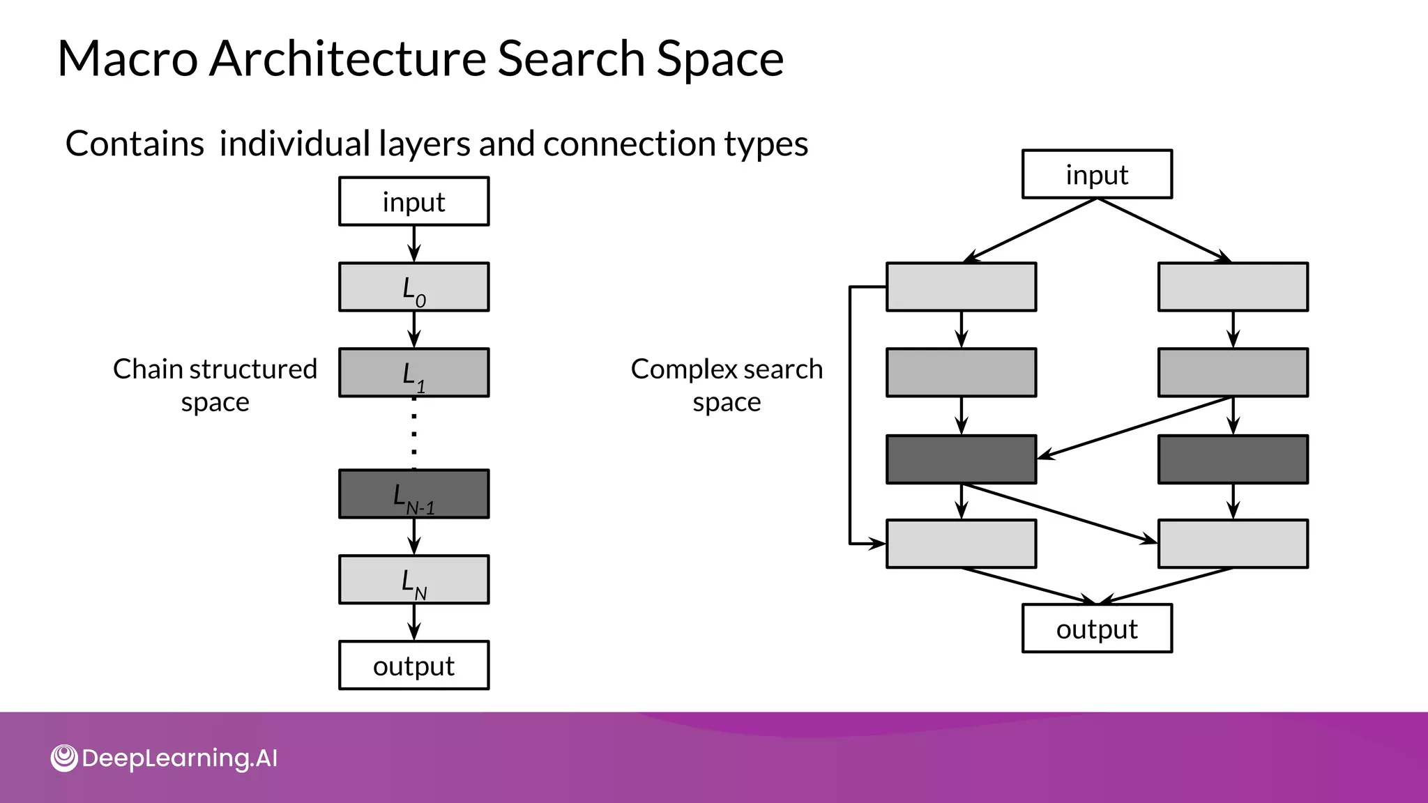
25. Neural Architecture Search
Search Space
A
Neural Architecture a ∈ A
Architecture is picked from
this space by search
strategy
Accuracy
Latency
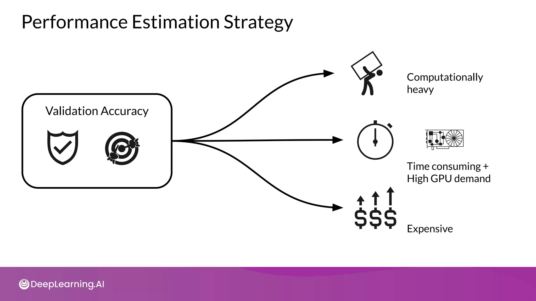
Performance Estimation Strategy
Performance
Search Strategy

26. Neural Architecture Search
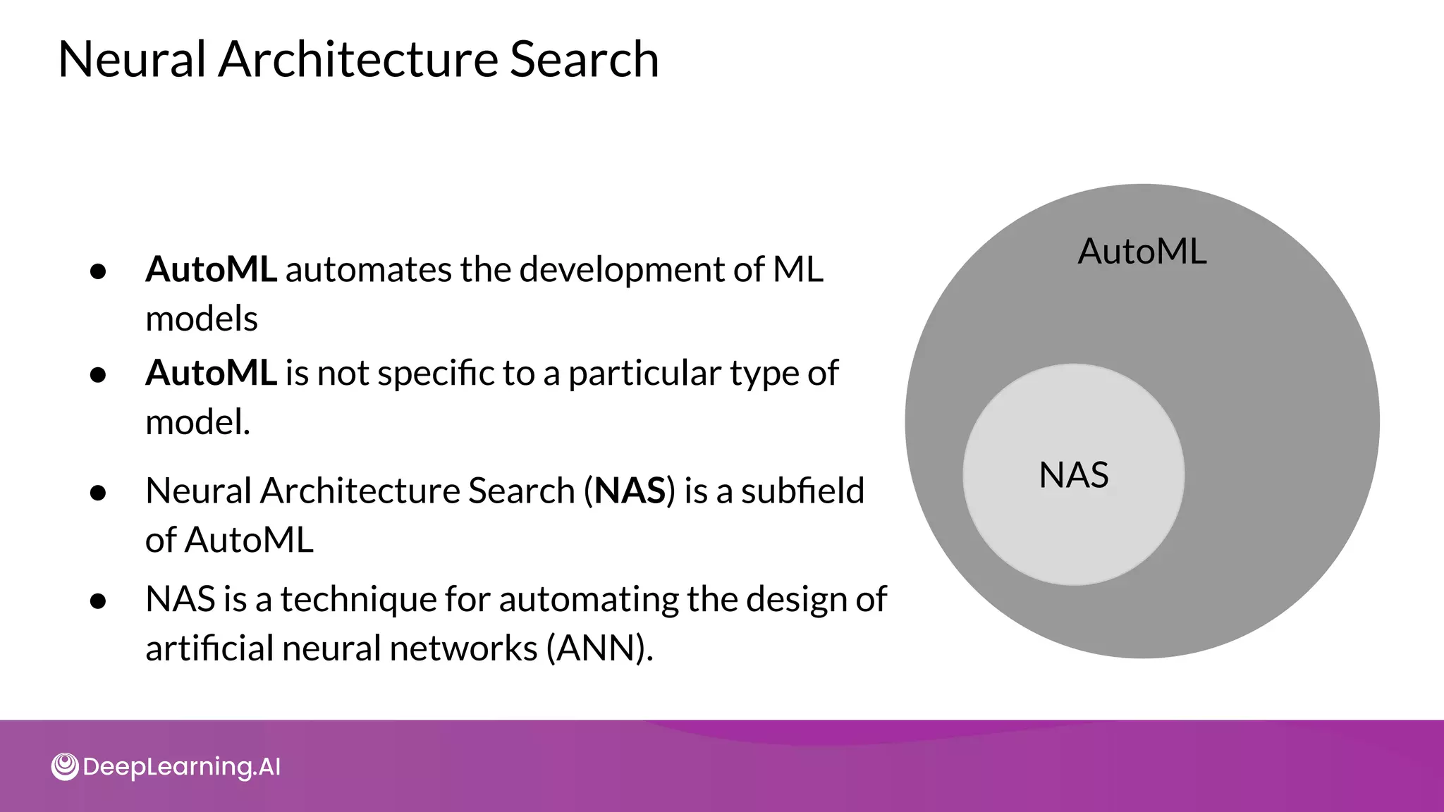
● AutoML automates the development of ML
models
● AutoML is not specific to a particular type of
model.
● NAS is a technique for automating the design of
artificial neural networks (ANN).
NAS
AutoML
● Neural Architecture Search (NAS) is a subfield
of AutoML

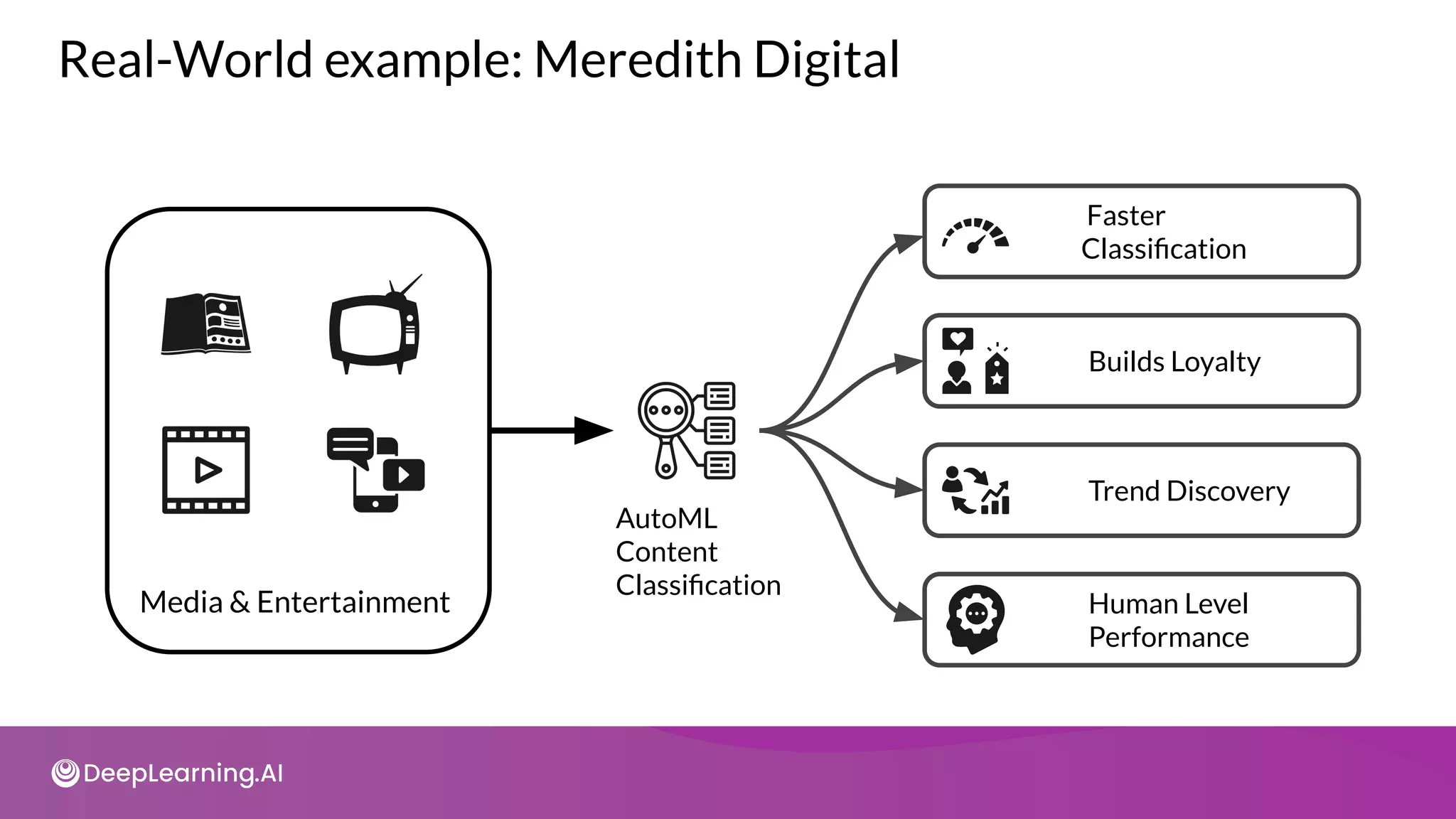
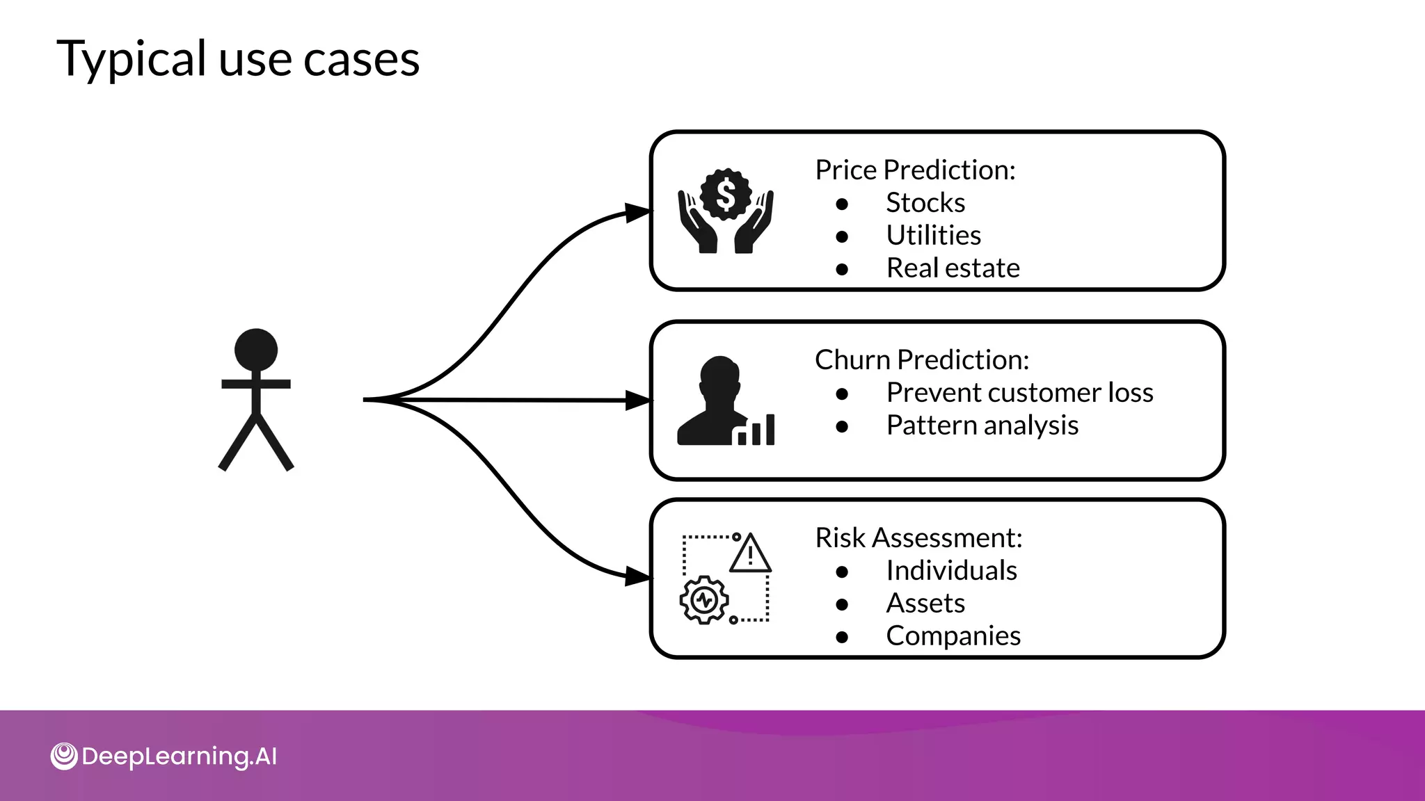
27. Real-World example: Meredith Digital
Media & Entertainment
AutoML
Content
Classification
Faster
Classification
Builds Loyalty
Trend Discovery
Human Level
Performance

28. AutoML
Understanding Search
Spaces

29. Types of Search Spaces
input
Macro
L0
L1
LN-1
LN
output
Li
Node
Connection
Micro
input
output

30. Macro Architecture Search Space
Contains individual layers and connection types
input
Chain structured
space
L0
L1
LN-1
LN
output
input
Complex search
space
output

31. Micro Architecture Search Space
Normal Cell
Reduction Cell
Repertoire
input
output
input
output
input
output
input

32. AutoML
Search Strategies

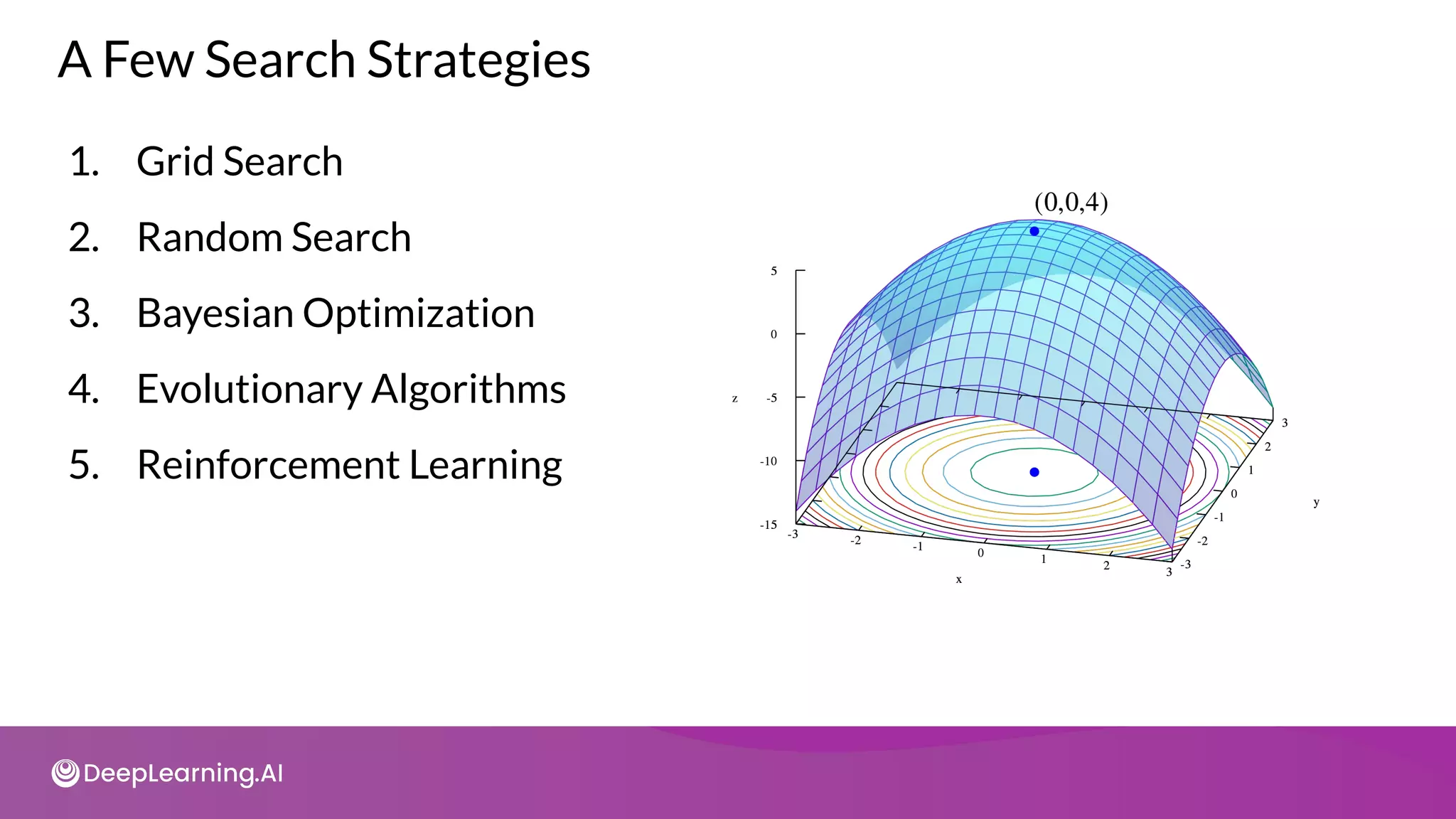
33. 1. Grid Search
2. Random Search
3. Bayesian Optimization
4. Evolutionary Algorithms
5. Reinforcement Learning
A Few Search Strategies

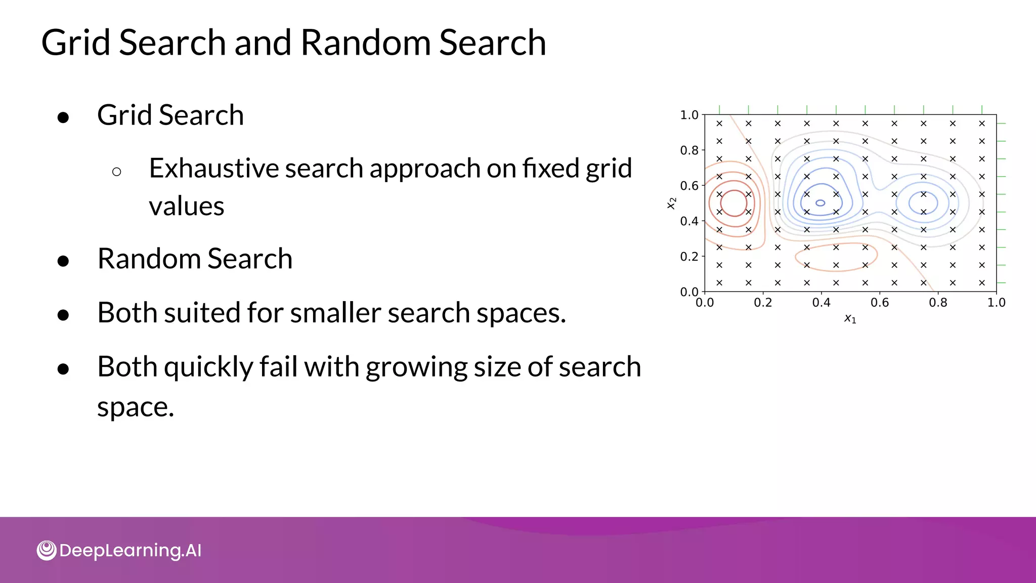
34. Grid Search and Random Search
● Grid Search
○ Exhaustive search approach on fixed grid
values
● Random Search
● Both suited for smaller search spaces.
● Both quickly fail with growing size of search
space.

35. Bayesian Optimization
● Assumes that a specific probability
distribution, is underlying the performance.
● Tested architectures constrain the
probability distribution and guide the
selection of the next option.
● In this way, promising architectures can be
stochastically determined and tested.

36. Parents Selected
Parents
Parents
+
Offspring
X
X X
Select
+
remove
Replace
with
offspring
Repeat
Evolutionary Methods

37. Reinforcement Learning
State
● The performance estimation
strategy determines the reward
Reward
● Agents goal is to maximize a
reward
Agent
● The available options are
selected from the search space Action
Search
space

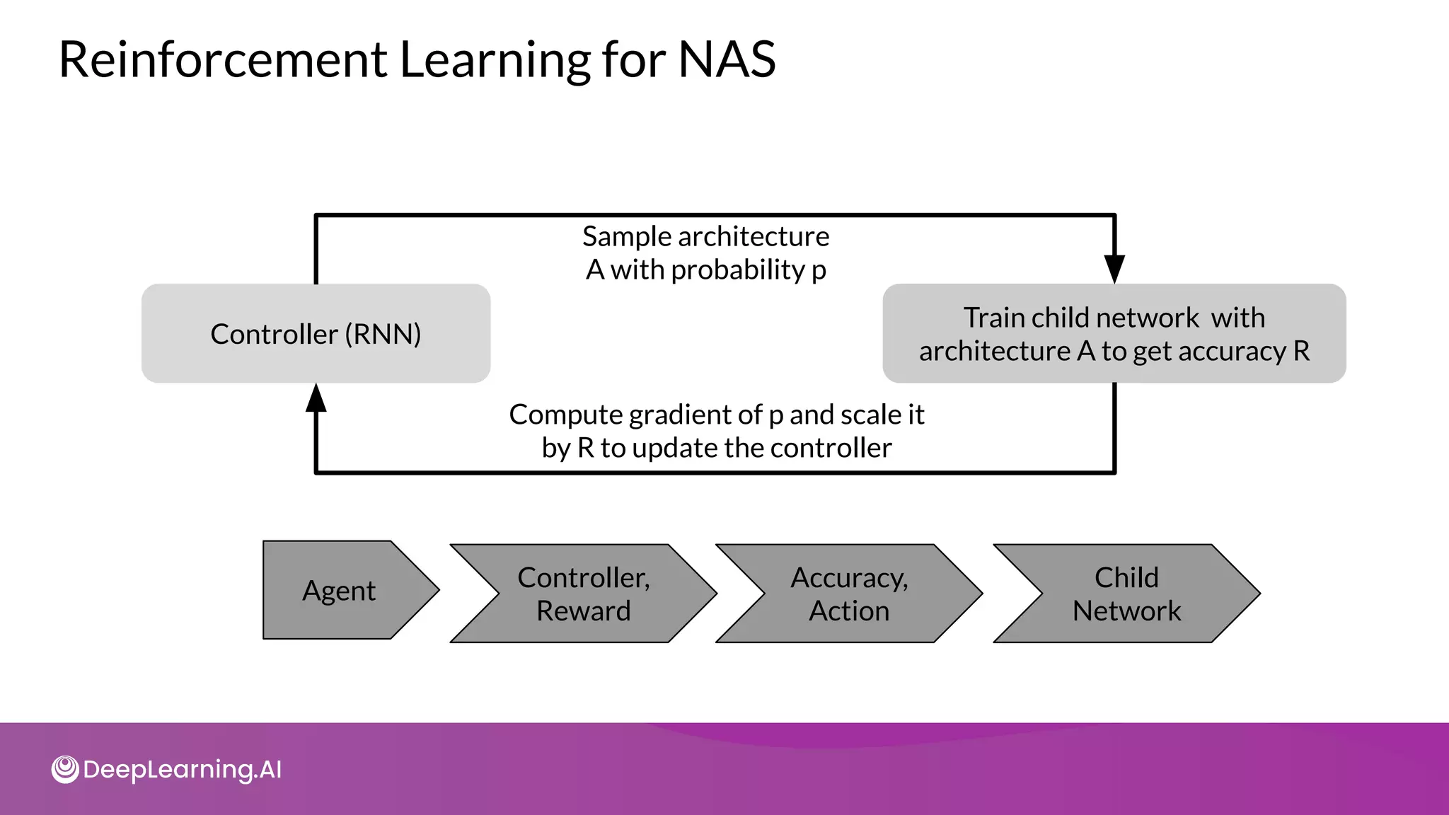
38. Controller (RNN)
Train child network with
architecture A to get accuracy R
Agent Controller,
Reward
Accuracy,
Action
Child
Network
Sample architecture
A with probability p
Compute gradient of p and scale it
by R to update the controller
Reinforcement Learning for NAS

39. AutoML
Measuring AutoML Efficacy

40. Validation Accuracy
Performance Estimation Strategy
Computationally
heavy
Time consuming +
High GPU demand
Expensive

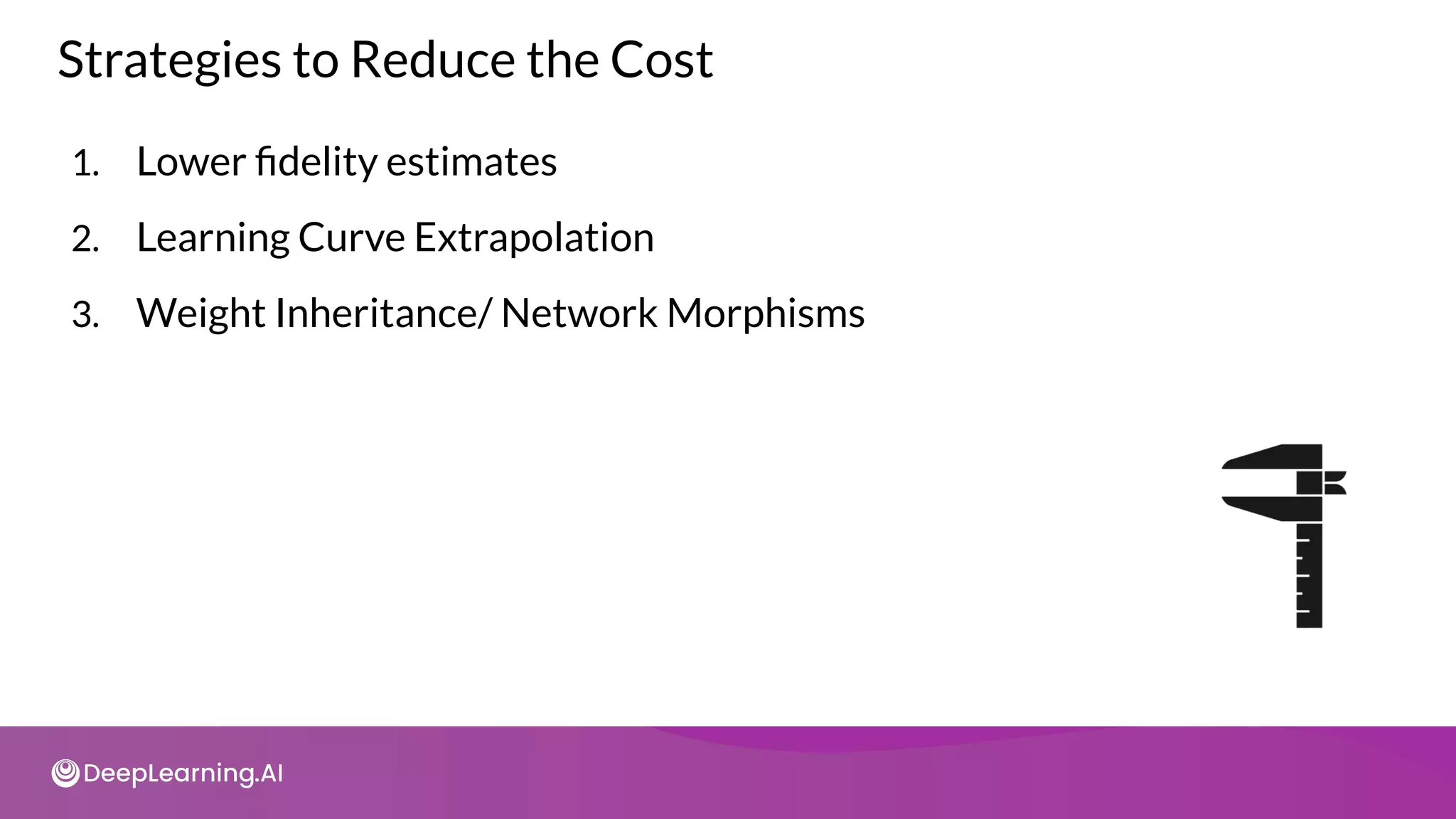
41. 1. Lower fidelity estimates
2. Learning Curve Extrapolation
3. Weight Inheritance/ Network Morphisms
Strategies to Reduce the Cost

42. Lower Fidelity Estimates
Reduce
training time
Data subset
Low resolution
images
Fewer filters
and cells
● Reduce cost but
underestimates performance
● Works if relative ranking of
architectures does not
change due to lower fidelity
estimates
● Recent research shows this
is not the case

43. Learning Curve Extrapolation
● Requires predicting the learning curve reliably
X
X
● Extrapolates based on initial learning.
● Removes poor performers

44. Weight Inheritance/Network Morphisms
● Initialize weights of new architectures based on previously trained
architectures
○ Similar to transfer learning
● Uses Network Morphism
● Underlying function unchanged
○ New network inherits knowledge from parent network.
○ Computational speed up: only a few days of GPU usage
○ Network size not inherently bounded

45. AutoML
AutoML on the Cloud

46. Popular Cloud Offerings
Cloud-based AutoML
Amazon SageMaker Autopilot
Microsoft Azure Automated Machine Learning
Google Cloud AutoML

47. Amazon SageMaker Autopilot

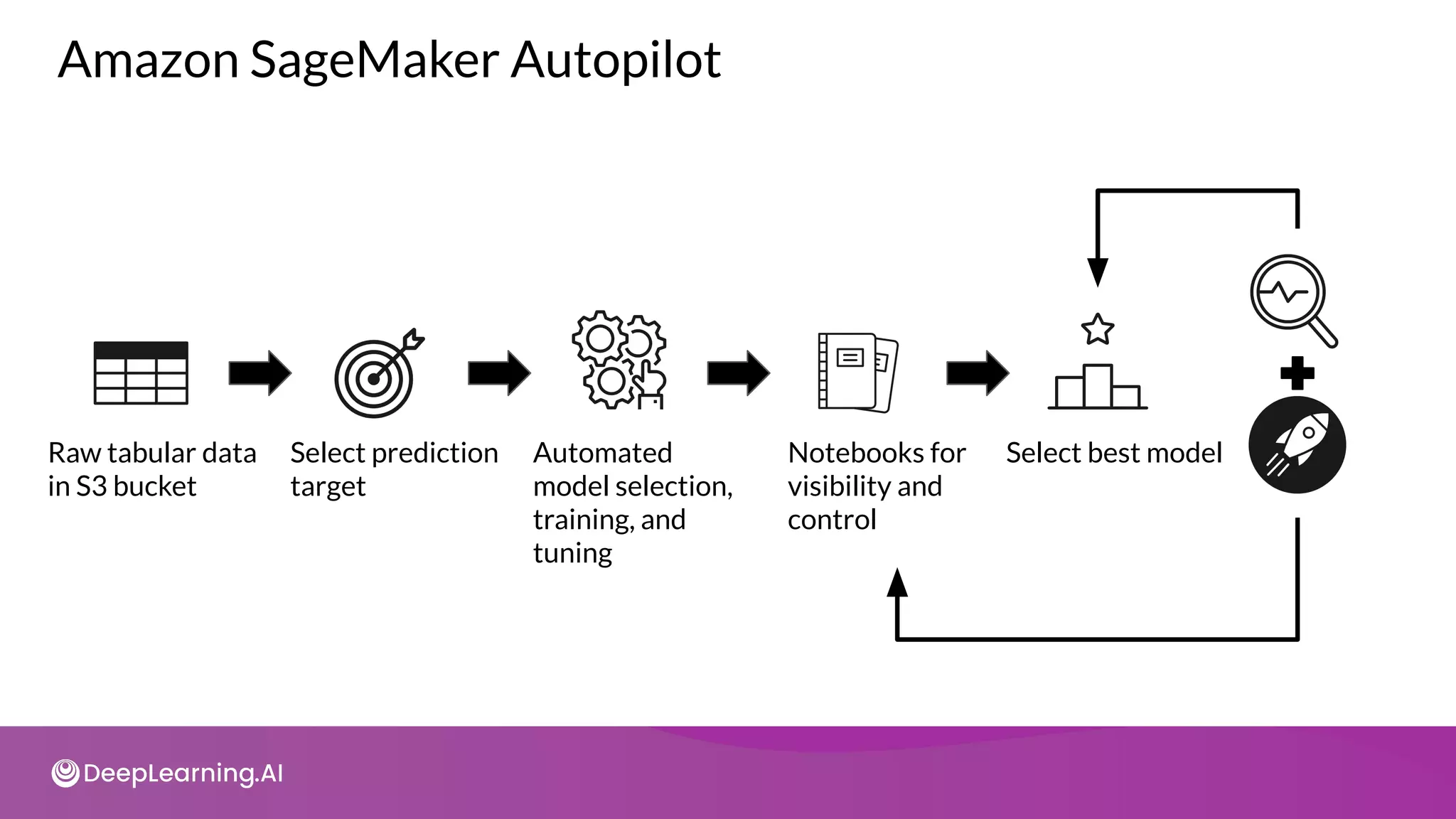
48. Amazon SageMaker Autopilot
Raw tabular data
in S3 bucket
Select prediction
target
Automated
model selection,
training, and
tuning
Notebooks for
visibility and
control
Select best model

49. Key features
Quick Iteration
High quality models
Performance ranked
Selected features
Notebooks for reproducibility

50. Typical use cases
Price Prediction:
● Stocks
● Utilities
● Real estate
Risk Assessment:
● Individuals
● Assets
● Companies
Churn Prediction:
● Prevent customer loss
● Pattern analysis

51. Microsoft Azure
Automated Machine Learning

52. Microsoft Azure AutoML
Automated Feature
Selection
Automated Model
Selection
Optimized model
Hyperparameter
Tuning

53. Key features
Quick customization:
● Model
● Control settings
Data Visualization
Automated Feature Engineering
Intelligent stopping

54. Key features
● Experiment summaries
● Metric visualizations
Model Interpretability
Pattern Discovery

55. Google Cloud AutoML

56. Google Cloud AutoML
● Accessible to beginners
● Train high-quality models
● GUI Based
● Pipeline life-cycle
● Neural Architecture Search
● Transfer Learning
● Data labeling
● Data cleaning

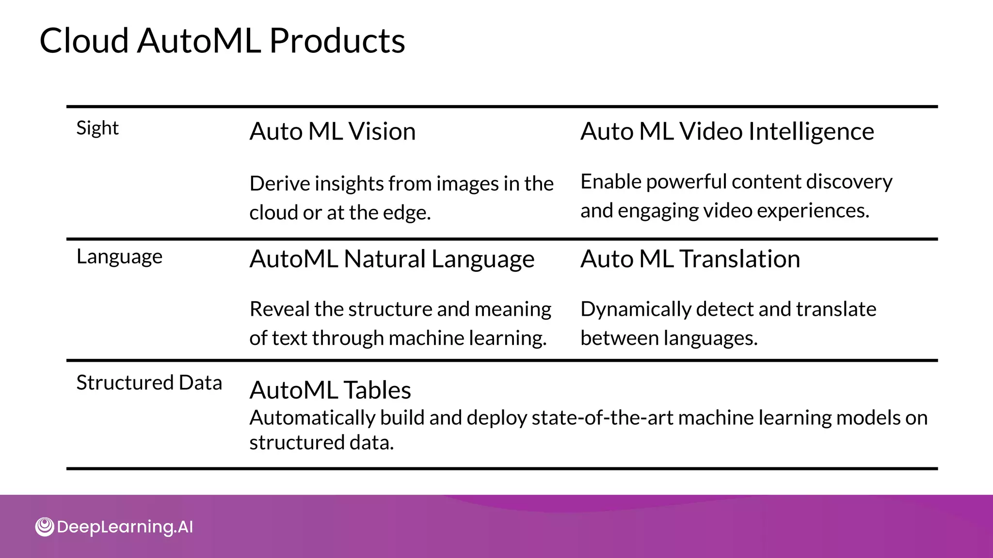
57. Structured Data AutoML Tables
Automatically build and deploy state-of-the-art machine learning models on
structured data.
Cloud AutoML Products
Sight Auto ML Vision
Derive insights from images in the
cloud or at the edge.
Auto ML Video Intelligence
Enable powerful content discovery
and engaging video experiences.
Language AutoML Natural Language
Reveal the structure and meaning
of text through machine learning.
Auto ML Translation
Dynamically detect and translate
between languages.

58. AutoML Vision Products
AutoML Vision Object Detection AutoML Vision Edge Object Detection
Auto ML Vision Classification AutoML Vision Edge Image Classification

59. AutoML Video Intelligence Classification
Enables you to train machine learning models, to classify shots and segments on
your videos according to your own defined labels.
AutoML Video Intelligence Products
AutoML Video Object detection
Enables you to train machine learning models to detect and track multiple
objects, in shots and segments.

60. So what’s in the secret sauce?
How do these Cloud offerings perform AutoML?
● We don’t know (or can’t say) and they’re not about to
tell us
● The underlying algorithms will be similar to what
we’ve learned
● The algorithms will evolve with the state of the art

61. AutoML
Assignment Setup

62. Setup
AutoML
1
Steps to Classify Images using AutoML Vision
2
Create
Dataset
Upload images to
Cloud Storage and
create dataset in
Vision.
3
Train Evaluate
4
Deploy
model for
serving
5
Deploy
6
Test
Generate
predictions using
deployed model

63. ● Qwiklabs provides real cloud environments that help developers and IT
professionals learn cloud platforms and software.
● Check tutorial on Qwiklabs basics
Setup
AutoML
1 2
Create
Dataset
3
Train Evaluate
4 5
Deploy
6
Test

64. It’s your turn!