The document discusses efficient techniques for deep learning on edge devices. It begins by noting that deep neural networks have high computational complexity which makes inference inefficient for edge devices without powerful GPUs. It then outlines the deep learning stack from hardware to libraries to frameworks to algorithms. The document focuses on how algorithms define model complexity and discusses the evolution of CNN architectures from LeNet5 to ResNet which generally increased in complexity. It covers techniques for reducing model size and operations like pruning, quantization, and knowledge distillation. The challenges of real-life applications on edge devices are discussed.

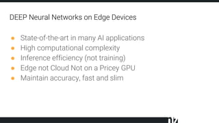
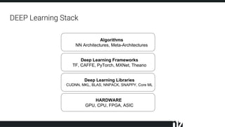
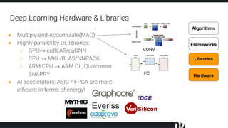
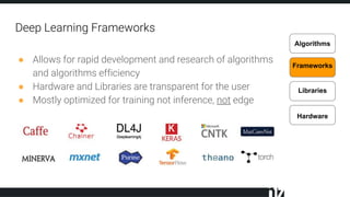
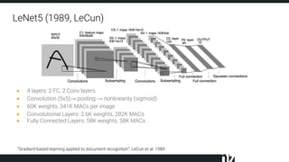
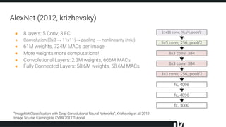
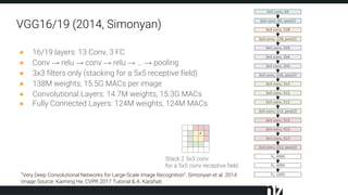
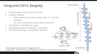
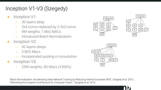
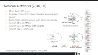
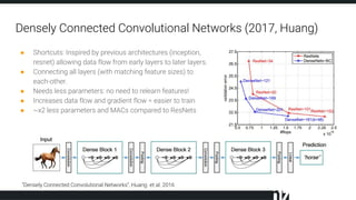
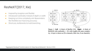
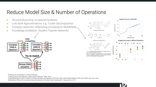
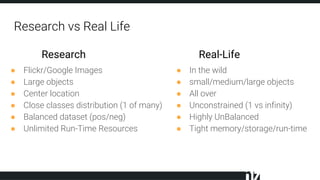
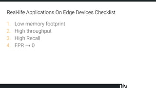
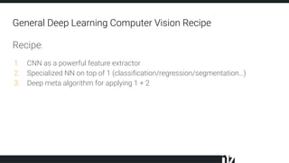
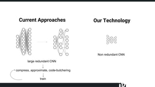
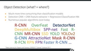
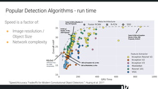
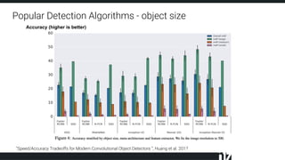
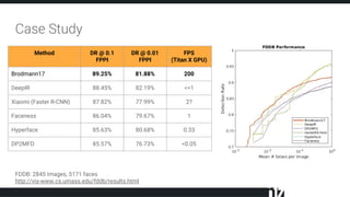
1. Efficient Deep Learning
Amir Alush, PhD

2. DEEP Neural Networks on Edge Devices
● State-of-the-art in many AI applications
● High computational complexity
● Inference efficiency (not training)
● Edge not Cloud Not on a Pricey GPU
● Maintain accuracy, fast and slim

3. DEEP Learning Stack
HARDWARE
GPU, CPU, FPGA, ASIC
Deep Learning Libraries
CUDNN, MKL, BLAS, NNPACK, SNAPPY, Core ML
Deep Learning Frameworks
TF, CAFFE, PyTorch, MXNet, Theano
Algorithms
NN Architectures, Meta-Architectures

4. Deep Learning Hardware & Libraries
Hardware
Libraries
Frameworks
Algorithms
● Multiply-and-Accumulate(MAC)
● Highly parallel by DL libraries:
○ GPU→ cuBLAS/cuDNN
○ CPU → MKL/BLAS/NNPACK
○ ARM CPU → ARM CL, Qualcomm
SNAPPY
● AI accelerators: ASIC / FPGA are more
efficient in terms of energy!
CONV
FC

5. Deep Learning Frameworks
Hardware
Libraries
Frameworks
Algorithms
● Allows for rapid development and research of algorithms
and algorithms efficiency
● Hardware and Libraries are transparent for the user
● Mostly optimized for training not inference, not edge

6. Deep Learning Algorithms
Hardware
Libraries
Frameworks
Algorithms
Have a crucial role in efficiency since algorithms
define the model’s complexity and size

7. Evolution of CNN
Architectures

8. LeNet5 (1989, LeCun)
● 4 layers: 2 FC, 2 Conv layers.
● Convolution (5x5)→ pooling → nonlinearity (sigmoid)
● 60K weights, 341K MACs per image
● Convolutional Layers: 2.6K weights, 282K MACs
● Fully Connected Layers: 58K weights, 58K MACs
“Gradient-based learning applied to document recognition”, LeCun et al. 1989

9. AlexNet (2012, krizhevsky)
● 8 layers: 5 Conv, 3 FC
● Convolution (3x3 → 11x11)→ pooling → nonlinearity (relu)
● 61M weights, 724M MACs per image
● More weights more computations!
● Convolutional Layers: 2.3M weights, 666M MACs
● Fully Connected Layers: 58.6M weights, 58.6M MACs
“ImageNet Classification with Deep Convolutional Neural Networks”, Krizhevsky et al. 2012
Image Source: Kaiming He, CVPR 2017 Tutorial

10. ● 16/19 layers: 13 Conv, 3 FC
● Conv → relu → conv → relu → … → pooling
● 3x3 filters only (stacking for a 5x5 receptive field)
● 138M weights, 15.5G MACs per image
● Convolutional Layers: 14.7M weights, 15.3G MACs
● Fully Connected Layers: 124M weights, 124M MACs
VGG16/19 (2014, Simonyan)
Stack 2 3x3 conv
for a 5x5 conv receptive field.
“Very Deep Convolutional Networks for Large-Scale Image Recognition”, Simonyan et al. 2014
Image Source: Kaiming He, CVPR 2017 Tutorial & A. Karphati

11. 1 fully connected
GoogLenet (2014, Szegedy)
“Going deeper with convolutions”, Szegedy et al. 2014
Image source: .”Efficient Processing of Deep Neural Networks: A Tutorial and Survey”, Sze et al.
9inceptionmodules
inception module
3 convolutions
● 21 layers deep: 57 Conv layers,1 FC layer
● Inception modules:
○ Multi-branching with Different filter sizes: 1x1, 3x3, 5x5
○ Shortcuts
○ 1x1 convs “bottleneck” used to reduce #channels
● 7M weights, 1.43G MACs per image
● Convolutional Layers: 6M weights, 1.43G MACs
● Fully Connected Layers: 1M weights, 1M MACs

12. Inception V1-V3 (Szegedy)
● Inception V1:
○ 30 layers deep
○ 5x5 convs replaced by 2 3x3 convs
○ 9M weights, 1.86G MACs
○ Introduced Batch Normalization
● Inception V2:
○ 42 layers deeps
○ 2.86G Macs
○ Incorporated pooling in convolution
● Inception V3:
○ 25M weights, 5G Macs (+200%)
“Batch Normalization: Accelerating Deep Network Training by Reducing Internal Covariate Shift”, Szegedy et al. 2015
“Rethinking the Inception Architecture for Computer Vision”, Szegedy et al. 2015

13. Residual Networks (2016, He)
“Deep Residual Learning for Image Recognition”, He et al. 2016
Residual building block
● More than 1000 layers
● Residual connections: more accurate, easier to train,
deeper
● Bottlenecks to make deeper with same complexity
● ResNet 34: 3.6G MACs
● ResNet 50: 3.8G MACs, 25M weights
● ResNet 152: 11.3G MACs

14. Densely Connected Convolutional Networks (2017, Huang)
● Shortcuts: Inspired by previous architectures (inception,
resnet) allowing data flow from early layers to later layers.
● Connecting all layers (with matching feature sizes) to
each-other.
● Needs less parameters: no need to relearn features!
● Increases data flow and gradient flow = easier to train
● ~x2 less parameters and MACs compared to ResNets
“Densely Connected Convolutional Networks”, Huang et al. 2016

15. ResNeXT(2017, Xie)
● Inspired by Inception and ResNet
● Introduced Cardinality instead of depth or width
● Keeping run-time complexity and #parameters
like ResNets but improving accuracy.
● Shortcuts, bottlenecks & multi-branching
“Aggregated Residual Transformations for Deep Neural Networks”, Xie et al. 2016

16. Architectures Thus Far...
● Accuracy is the highest
priority for most researchers,
even when able to reduce
computations, deeper more
complex models are used!
● CNNs complexity Increases
● MACs increases
“An Analysis of Deep Neural Network Models for Practical Applications”, Canziani et al. 2017

17. Fitting to Hardware

18. Reduce Model Size & Number of Operations
● Pruning redundant weights and retrain (a.k.a “Brain Damage”):
○ According to some criteria: impact on training-loss, energy
○ Simply remove small weights
● Custom hardware to support sparse matrix multiplications: e.g. EIE
”Optimal Brain Damage”, LeCun et al. 1990
“Designing Energy-Efficient Convolutional Neural Networks using Energy-Aware Pruning “, Yang et al. 2017
“Learning both weights and connections for efficient neural networks”, Yang et al. 2015
“EIE: efficient inference engine on compressed deep neural network”, Han et al. 2016

19. Reduce Model Size & Number of Operations
● Structured pruning: no special hardware
● Low Rank Approximations: e.g. Tucker Decomposition
● Compact networks: refactoring convolutions: MobileNets
● Knowledge Distillation: Student-Teacher Networks
“Distilling the Knowledge in a Neural Network
“Learning structured sparsity in deep neural networks“, Wen, 2016
“COMPRESSION OF DEEP CONVOLUTIONAL NEURAL NETWORKS FOR FAST AND LOW POWER MOBILE APPLICATIONS”, Kim et al. 2016
“MobileNets: Efficient Convolutional Neural Networks for Mobile Vision Application”, Howard et al. 2017

20. Reduce Precision (quantization) of Weights & Activations
● 32-bit float → 16 / 8 / 4 / 2 / 1 -bit fixed-point
● Weights/Activations quantization: reduces storage / computation
● Different schemes: linear, non-linear, clustering (weight sharing)
● Can be fixed / variable (depending on weights, activations, layers, channels distribution)
● Reduces processing time!
● Decreases accuracy, Re-training helps
”Efficient Processing of Deep Neural Networks: A Tutorial and Survey”, Sze et al. 2017

21. Brodmann17

22. Research vs Real Life
Research Real-Life

23. Research vs Real Life
● Flickr/Google Images
● Large objects
● Center location
● Close classes distribution (1 of many)
● Balanced dataset (pos/neg)
● Unlimited Run-Time Resources
● In the wild
● small/medium/large objects
● All over
● Unconstrained (1 vs infinity)
● Highly UnBalanced
● Tight memory/storage/run-time
Research Real-Life

24. Real-life Applications On Edge Devices Checklist
1. Low memory footprint
2. High throughput
3. High Recall
4. FPR → 0

25. General Deep Learning Computer Vision Recipe
Recipe:
1. CNN as a powerful feature extractor
2. Specialized NN on top of 1 (classification/regression/segmentation…)
3. Deep meta algorithm for applying 1 + 2

26. Current Approaches Our Technology
large redundant CNN
Non redundant CNN
compress, approximate, code-butchering
train

27. Object Detection (what? + where?)
● Much more time consuming than classification models
● Detection CNN = CNN feature extractor + Regression/Classification NN
● Numerous popular algorithms exist today:
”Deep Learning for Objects and Scenes, CVPR2017 Tutorial”, Girshick 2017

28. ”Speed/Accuracy Tradeoffs for Modern Convolutional Object Detectors ”, Huang et al. 2017
Popular Detection Algorithms - run time
Speed is a factor of:
● Image resolution /
Object Size
● Network complexity

29. Popular Detection Algorithms - object size
”Speed/Accuracy Tradeoffs for Modern Convolutional Object Detectors ”, Huang et al. 2017
Accuracy (higher is better)

30. Case Study
Method DR @ 0.1
FPPI
DR @ 0.01
FPPI
FPS
(Titan X GPU)
Brodmann17 89.25% 81.88% 200
DeepIR 88.45% 82.19% <=1
Xiaomi (Faster R-CNN) 87.82% 77.99% 2?
Faceness 86.04% 79.67% 1
Hyperface 85.63% 80.68% 0.33
DP2MFD 85.57% 76.73% <0.05
FDDB: 2845 images, 5171 faces
http://vis-www.cs.umass.edu/fddb/results.html

31. Looking for brilliant
researchers
cv@brodmann17.com
Nir
Netanell
Ben
Ben
Yossi
Shai
30 FPS on 1xA72!