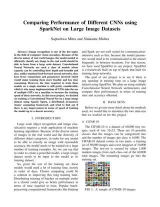
This document discusses comparing the performance of different convolutional neural networks (CNNs) when trained on large image datasets using Apache Spark. It summarizes the datasets used - CIFAR-10 and ImageNet - and preprocessing done to standardize image sizes. It then provides an overview of CNN architecture, including convolutional layers, pooling layers, and fully connected layers. Finally, it introduces SparkNet, a framework that allows training deep networks using Spark by wrapping Caffe and providing tools for distributed deep learning on Spark. The goal is to see if SparkNet can provide faster training times compared to a single machine by distributing training across a cluster.

1. Comparing Performance of Different CNNs using
SparkNet on Large Image Datasets
Saptashwa Mitra and Sitakanta Mishra
Abstract— Image recognition is one of the hot topics
in the field of computer vision nowadays. Because of the
diverse nature of real world images, the model needed to
efficiently classify any image in the real world should be
able to learn from a large scale dataset. Convolutional
Neural Networks are such a class of models whose
capacity can be controlling their depth and breadth and
also, unlike standard feed-forward neural networks, they
have fewer connections and parameters involved which
would make training them more feasible and less time
consuming. However, the time required to train these
models on a single machine is still pretty considerable,
which is why many implementations of CNNs take the use
of multiple GPUs on a machine to increase the training
speed of these networks. In this term project, we decided
on training a Convolutional Neural Net on a large image
dataset using Apache Spark, a distributed, in-memory
cluster computing framework and tried to find out if
there is any improvement in terms of speed of training
the model up to a decent accuracy.
I. INTRODUCTION
Large scale object recognition and image clas-
sification requires a wide application of machine
learning algorithms. Because of the diverse nature
of images in the real world and the diversity of
different object categories, in order for any model
to be able to classify an image with reasonable
accuracy, the model needs to be trained on a large
number of training examples. So, we can say that
in order to create a powerful model, a large image
dataset needs to be input to the model as its
training dataset.
So, given the size of the training set, these
models would need a lot of training time, mostly
in order of days. Cluster computing could be
a solution to improving this long training time.
Distributing training of batches on multiple nodes
in a cluster could give us better performance in
terms of time required to train. Popular batch-
processing computational frameworks like Hadoop
and Spark are not well suited for communication-
intensive such as this, because the model parame-
ters would need to be communicated to the master
frequently in between iterations. For that reason,
we have used SparkNet in our project. SparkNet
is a framework built on top of Spark that built for
training deep networks.
The goal of our project is to see if there is
any speedup in training time on a large image
dataset using SparkNet. We plan on using multiple
Convolutional Neural Network architectures and
compare their performances in terms of training
time and accuracy obtained.
II. DATA SETS
Before we go into more detail about the methods
used, we would like to introduce the two data-sets
that we worked on for this project.
A. CIFAR-10
The CIFAR-10 is a dataset of 60,000 tiny im-
ages, each of size 32x32. There are 10 possible
classes that the images can be categorized into
and the number of images per class is 6,000. The
CIFAR-10 dataset comes in two parts, a training
set of 50,000 images and a test imageset of 10,000
images. The test-set is created by taken 1,000
random images from each class out of the 60,000
total images. The remaining images go into the
training set.
FIG 1:. A sample of CIFAR-10 images

2. B. IMAGENET
ImageNet is a dataset of more than 1.2 million
images meant to be used in object recognition
research. This dataset has been the subject of the
ILSVRC challenge since 2010. The goal is to
correctly as little error rate on classification of
these images as possible. The training set itself
is about 1.2 million images and the validation set
consists of 50,000 images and the test set contains
100,000 images. Both the training and validation
imageset come with a text file identifying each
image filename to its corresponding category. A
test dataset of 150,000 images is also provided in
the imagenet data. The images in this dataset are
not of any fixed size and can be large images. We
have used the Imagenet dataset from 2012, which
has a total size of over 150 gb.
FIG 2:. A sample of Imagenet images
III. METHODS
Convolution Neural Networks have emerged as
the forerunners when it comes to classifying large
image datasets. Over the years, all the winners of
the ILSVRC competitions have come up with some
variation of a CNN model. Although simple learn-
ing tasks on smaller datasets can be easily done
without the use of CNNs, classifying thousands or
millions of images requires a training model with
a large training capacity.
Also, the immense complexity of the object
recognition task means that this problem cannot
be specified even by a large, so our model should
also have lots of prior knowledge to compensate
for all the data we dont have as explained below.
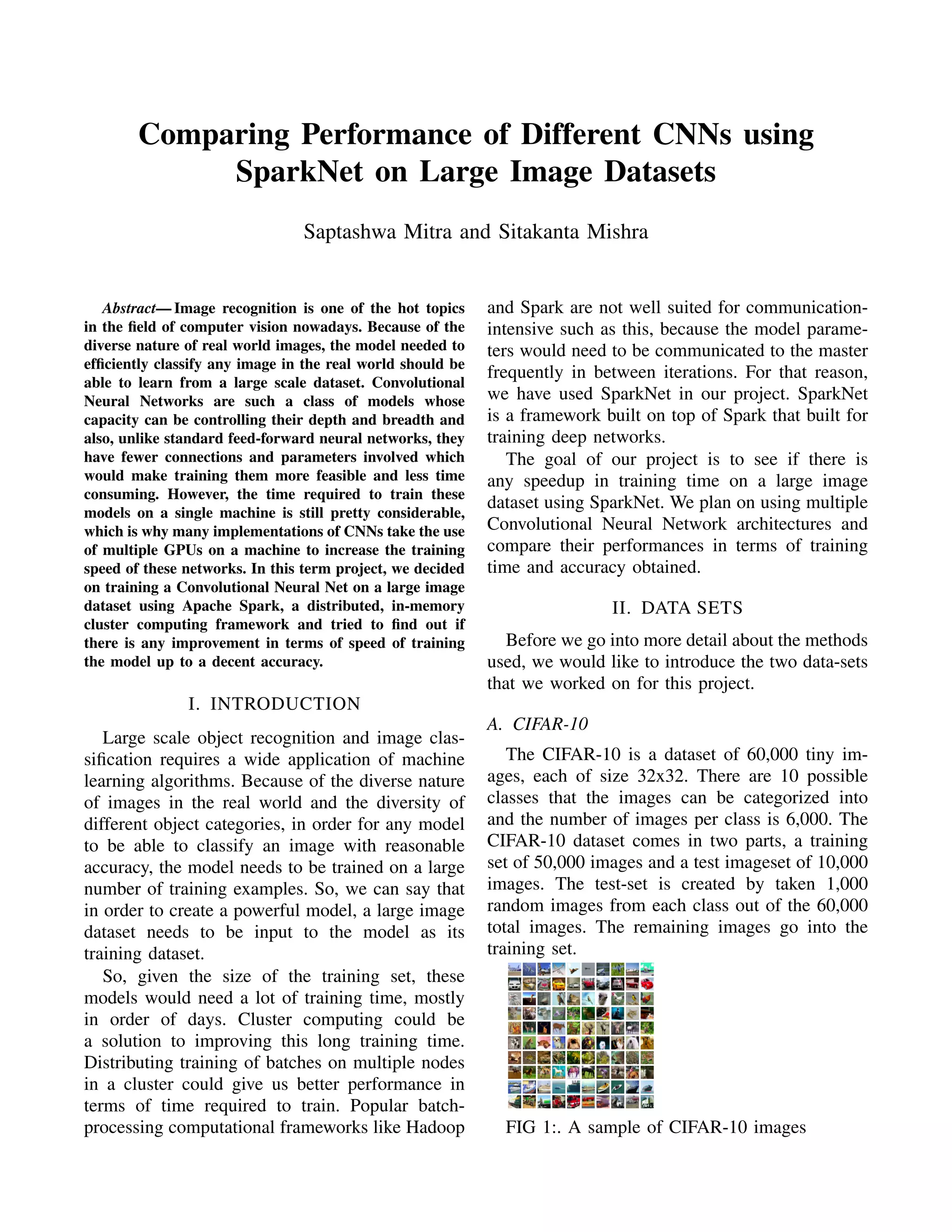
A. Data Preprocessing
Our software requires the images to be input
at a fixed dimension. Cifar-10s images are all of
the same dimension. But, since the input images
of ImageNet are varying in resolution, we have
used the method used in AlexNets[1] paper to get
around the problem.
Here, we down-sampled the images to a fixed
resolution of 256 x 256. Given a rectangular image,
we first rescaled the image such that the shorter
side was of length 256, and then cropped out the
central 256 x 256 patch from the resulting image.
These images are to be treated as input to our
model. During training also, our model takes a 227
x 227 random crop of each input image to avoid
overfitting.
B. Convolutional Neural Networks
Convolutional Neural Networks (CNN) are a
specialized type of neural network that are de-
signed to train large sized training data having a
grid-like topology. Image data fit this description
perfectly.
A convolution network is a specialized type of
neural network that prefers convolution instead on
general matrix multiplication. CNN architecture
make the explicit assumption that the inputs are
images, which allows us to encode certain prop-
erties into the architecture. These then make the
forward function more efficient to implement and
vastly reduce the amount of parameters in the
network.
Since for regular neural network, each neuron
in one layer is fully connected to neurons in the
previous layer, the problem at hand would become
very complicated and time consuming if regular
neural networks were used, simply because of the
huge number of parameters that would be involved
in the training process.
A convolution Network consists of a sequence
of layers. The purpose of these layers is to take
one volume of input activations and convert them
into output activations. There are three main types
of layers that are used to build ConvNet archi-
tectures: Convolutional Layer(CONV), Pooling
Layer(POOL), and Fully-Connected Layer (FC,
exactly as seen in regular Neural Networks). These
layers get stacked in different combinations to get
different implementations of a ConvNet architec-
ture that we see today.
Convolutional Layer: The CONV layers pa-
rameters consist of a set of learnable filters. Every
filter is small spatially (along width and height),
but extends through the full depth of the input
volume. During the forward pass, we slide (con-
volve) each filter across the width and height

3. of the input volume and compute dot products
between the entries of the filter and the input
at any position. As we slide the filter over the
width and height of the input volume we will
produce a 2-dimensional activation map that gives
the responses of that filter at every spatial position.
Following is an example of how multiple activation
maps from using multiple filters can be clubbed
together to form an input for the next stage of a
CNN. Each convolution layer is also followed by
an elementwise activation function (ReLU).
FIG 3:. An example of Convolutional layer
Mathematically we can say, a convolution
layer:
• Accepts a volume of size W1xH1xD1
• Requires four hyperparameters
– Number of filters (K)
– Spatial extent of the filters (F)
– Stride (S)
– Size of zero Padding (P)
• Produces an output of dimension
W2xH2xD2 where:
– W2 = (W1F + 2P)/S + 1W2 =
(W1F + 2P)/S + 1
– H2 = (H1F + 2P)/S + 1
– D2 = K
Pooling Layer: Periodically, in between each
convolution layers, we insert Pooling Layers. The
purpose of pooling layers is to down-sample the
volume spatially.
A pooling function replaces the output of the
net at certain location with a summary statistic of
its nearby outputs. We have used max-pooling for
our experiment. In the Max-pooling operation, the
maximum output of a rectangular area is reported.
Pooling helps us to achieve invariance to trans-
formation as well as invariance to inputs of varying
size.
Fully Connected Layer: Neurons in a fully
connected layer have full connections to all ac-
tivations in the previous layer, as seen in regular
Neural Networks. Their activations can hence be
computed with a matrix multiplication followed by
a bias offset. The final layer of a CNN must always
be fully connected.
FIG 4:. An example of Max Pooling
So essentially, a CNN is just a sequence of the
following structure:
INPUT− > [[CONV − > RELU] ∗ N− >
POOL?] ∗ M− > [FC− > RELU] ∗ K− > FC
C. SparkNet
As mentioned before, for our project we have
worked with SparkNet, which is a framework for
training deep networks in Spark. It includes a
convenient interface for reading data from Spark
RDDs, a Scala interface to the Caffe deep learning
framework and lightweight multidimensional ten-
sor library. It builds on Apache Spark and the Caff
deep learning library.
In the implementation, the Net class wraps Caffe
and exposes a simple API containing methods. The
NetParams type specifies a network architecture
and the weightCollection type is map from layer
names to list of weights. It allows the manipu-
lation of network components and the storage of
weights and outputs for individual layers. NDArray
class, which is a lightweight multi-dimensional
tensor library which facilitates manipulation of
data and weights without copying memory from
Caffe. Spark consists of a single master node and
a number of worker nodes. The data is split among
the Spark workers. In every iteration, the Spark
master broadcasts the model parameters to each
worker. Each worker runs SGD on the model with
its subset of data for a fixed number of iterations
or for a fixed length of time. Then the resulting
model parameters on each worker are sent to
the master and averaged to form the new model
parameters.[3]

4. Caffe provides us with a specific format to
specify a CNN architecture to the program. Using
this format, we have specified the different CNN
architecture we have used. The following is a
sample code for specifying the protocol for a layer:
FIG 5:. Layer Specification on Caffe
D. Different CNN architecture
Some popular CNN architecture that we at-
tempted to implement were:
For ImageNet dataset:
Alexnet
[227x227x3]INPUT
[55x55x96]CONV 1 :
9611x11filtersatstride4, pad0
[27x27x96]MAXPOOL1 :
3x3filtersatstride2
[27x27x96]NORM1 : Normalizationlayer
[27x27x256]CONV 2 :
2565x5filtersatstride1, pad2
[13x13x256]MAXPOOL2 :
3x3filtersatstride2
[13x13x256]NORM2 : Normalizationlayer
[13x13x384]CONV 3 :
3843x3filtersatstride1, pad1
[13x13x384]CONV 4 :
3843x3filtersatstride1, pad1
[13x13x256]CONV 5 :
2563x3filtersatstride1, pad1
[6x6x256]MAXPOOL3 :
3x3filtersatstride2
[4096]FC6 : 4096neurons
[4096]FC7 : 4096neurons
[1000]FC8 : 1000neurons(classscores)
For Cifar-10
We were not able to implement AlexNet due to
reasons mentioned later. As a result, we decided
to train a set of different CNN architecture on the
Cifar-10 dataset. We tested out 2 CNNs on the
Cifar-10 dataset to see which one trained faster
and which one gave a better accuracy after a
certain number of iterations. The following are the
architecture we tried out on Cifar-10:
Trial #1:
32x32x3INPUT
CONV 1 : 5x5x3filtersatstride1, pad2
MAXPOOL1 : 3x3filtersatstride2
CONV 2 : 5x5x3filtersatstride1, pad2
ReLU
AV GPOOL2 : 3x3filtersatstride2
CONV 3 : 5x5x3filtersatstride1, pad2
ReLU
AV GPOOL3 : 3x3filtersatstride2
FC(SoftMax)
FC
FC(Softmaxwithloss)[10neurons]
Trial #2:
32x32x3INPUT
CONV 1 : 5x5x3filtersatstride1, pad2
MAXPOOL1 : 3x3filtersatstride2
CONV 2 : 5x5x3filtersatstride1, pad2
ReLU
AV GPOOL2 : 3x3filtersatstride2
CONV 3 : 5x5x3filtersatstride1, pad2
ReLU
AV GPOOL3 : 3x3filtersatstride2
CONV 4 : 5x5x3filtersatstride1, pad2
ReLU
AV GPOOL4 : 3x3filtersatstride2
FC(SoftMax)
FC
FC(Softmaxwithloss)[10neurons]
IV. RESULTS AND DISCUSSION
A. Working with ImageNet
We encountered a roadblock while training the
ImageNet dataset on a spark cluster we created
on the CS120 lab machines. We had added 23
nodes on our cluster, deployed Spark on them and
installed SparkNet on top. However, the job that
we submitted failed after running for a few hours.
We received RPC timeout exception on sub-
mitting our jobs. We believe it has to do with

5. the Master process not being able to accumulate
results from worker tasks on Spark. We noticed
that while running their respective tasks, some of
the worker nodes got disconnected midway leading
to the master not getting a heartbeat from the
worker processes which led to the failure.
So, specifically, workers handling large amount
of data were sometimes going offline for some
reason. We believe this problem is with the CS120
machines and the problem would not occur if we
used Spark on EC2 machines instead of the CS120
machines.
B. Working with Cifar-10 data
We had better luck training the Cifar-10 datset
with the two CNN architectures we mentioned
before. We logged the training time, iterations re-
quired and the accuracy achieved with the test data
after each iteration for both the implementations.
The following are the results we obtained:
FIG 6:. Plotting Accuracy vs. Time
FIG 7:. Plotting Accuracy vs. Training Iterations
We found that with an extra layer of CONV-
RELU-POOL in layer 4 for the Trial#2, we get
better accuracy over time. The training is faster
for Trial#2 that for Trial#1. We also see that for
a fixed number of iterations, the accuracy score
of the CNN with an extra layer is better than the
other.
V. CONCLUSION
Although CIFAR-10 is a far smaller dataset than
the ImageNet dataset, we believe that the conclu-
sions we draw from the CIFAR dataset could be
applied to ImageNet data as well. The tensorflow
site mentions that with Cifar, they achieved an
86% accuracy with almost 300k iterations. We
notice our model achieving nearly 80% accuracy
on the training set after about an hour with only
4k iterations. So we believe that training a CNN
on a large dataset could actually be beneficial on
SparkNet.
VI. FUTURE WORK
Our future work would include getting the
SparkNet to be able to train ImageNet dataset on
the CS120 machines. If the problems persist, EC2
clusters could be a good solution. The reason we
did not use EC2 for our class project was due to
the cost that would be involved due to charge for
data transfer to and within the clusters.
Once SparkNet is able to train on ImageNet
dataset, the next step would be to test out different
implementations of CNNs starting from AlexNet,
ZFNet etc. on the same cluster and compare their
performance based on the time it takes to train
the models and the accuracy obtained through
iterations.
A study on the accuracy of the different models
could also be done based on the top 5 scores on the
test dataset and using that data, we could determine
which of these models take less time and give
sufficiently less error rate on classifying the test
dataset.
VII. CONTRIBUTION
Installation of Spark and SparkNet was done by
SitaKanta. Data pre-processing was done by both
Saptashwa and Sitakanta. The training of the data
set was done by Saptashwa. The testing and valida-
tion was done by Sitakanta. The final project report
was majorly done by Saptashwa. Some editing was
done by Sitakanta. The poster presentation was
prepared by Sitakanta. Debugging of issues and

6. bugs were fixed with equal contribution of both
the team mates.
REFERENCES
[1] 1. Alex Krizhevsky; Ilya Sutskever; Geoffrey E. Hinton.
”ImageNet Classification with Deep Convolutional Neural
Networks”.
[2] http://cs231n.github.io/convolutional-networks/
[3] Philipp Moritz; Robert Nishihara; Ion Stoica; Michael I.
Jordan . ”SPARKNET: TRAINING DEEP NETWORKS IN
SPARK”.
[4] https://arxiv.org/pdf/1311.2901v3.pdf
[5] http://ieeexplore.ieee.org/stamp/stamp.jsp?arnumber=7753615
[6] Matei Zaharia, Mosharaf Chowdhury, Michael J. Franklin,
Scott Shenker, Ion Stoica Spark: Cluster Computing with
Working Sets
[7] https://www.cs.toronto.edu/ kriz/learning-features-2009-
TR.pdf
[8] http://image-net.org/