1. Introduction:
The
main
purpose
of
exploring
and
modelling
the
process
heat
transfer
of
heat
exchanger
would
be
increasing
total
efficiency
of
the
unit.
In
this
project
we
would
like
investigate
the
results
of
analytical
and
numerical
solution
with
the
results
of
modelling
and
simulation
process
of
a
tube
heat
exchanger.
The
whole
process
of
this
project
would
be
creating
two
different
procedure
with
MATLAB
and
FLUENT.
In
house
MATLAB
software
will
be
used
to
numerically
model
the
heat
transfer
procedure.
On
the
other
hand,
the
tube
will
be
designed
in
GAMBIT
software
before
importing
in
FLUENT
commercial
software.
Results
of
fluid
dynamic
computation
can
be
obtained
in
each
of
FLUENT
or
ANSYS/FLUENT
software.
Basics
of
Heat
Exchanger
Theory:
The
current
geometry
in
2-­‐D
can
be
simplified
as
the
following
picture
of
figure.1.
It
means
that
in
2-­‐D
we
can
have
a
similar
3-­‐D
model
and
there
is
a
total
axis-­‐symmetry
around
the
heat
exchanger.
Therefore,
we
can
define
and
evaluate
our
model
in
longitudinal
and
peripheral
directions.
In
2-­‐D
sketch
outer
layers
and
outer
walls
have
no
heat
transfers.
Therefore,
the
boundary
condition
of
Q=0
will
be
applied
in
this
area.
Air
with
ambient
temperature
of
300o
C
enters
through
the
second
layer
between
two
pipes
with
constant
velocity
and
one
of
the
project’s
targets
is
to
find
its
profile
in
steady-­‐state
condition.
Wall
temperature
in
inner
pipe
has
a
constant
700o
C
temperature,
and
conduction
is
the
only
way
of
heat
transfer.
Figure
1:
2D
sketch
for
heat
exchanger.
In
order
to
model
the
process
in
2-­‐D
or
3-­‐D
scheme,
we
can
have
still
more
simplification
for
our
geometry;
main
axis
at
the
middle
of
our
pipes
can
be
used
as
another
symmetry
line.
In
3-­‐D
modelling
we
use
a
quarter
of
all
geometry,
it
contains
double
symmetry.
The
bulk
velocity
for
inlet
of
the
second-­‐
layer
pipe
can
be
easily
calculated.
With
respect
to
turbulent
Reynolds
number,
pipe’s
hydraulic
diameter
and
required
fluid’s
properties
we
can
calculate
the
bulk
velocity
(Ub)
as
follows:
Hydraulic Diameter = 4*(Hydraulic Radius), (1)

2. Hydraulic Radius = (Projection Area)/(Peripheral Length) (2)
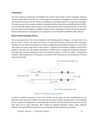
Equate Diameter = Outer Diameter – Inner Diameter = ( Do – Di ) (3)
Re = (Ub * Density * Deq) / (Dynamic Viscosity) (4)
Required Constants: Density = 1e5/287T= 0.596 [kg/m^3] (5), (6)
&
Dynamic Viscosity=1.747*10-5
+4.404*10-5
t –1.645*10-10
t2
=29.725*10-6
[kg/ms]
Re= 50000 => Ub = 50 m/s
Equations
and
Boundary
Conditions:
Three
different
ODE
(Ordinary
Differential
Equations)
can
feature
the
main
aspects
of
turbulent
theory.
We
can
say
that
between
ri<r<ro
the
following
equations
are:
!"
!"
=
!!
µ!!!!
!!
! !!!
!!
! !!!
!
∙ (
!!
!
) ri<r<rm
(7.a)
!"
!"
=
!!
µ!!!!
!!!!!
!
!!
!!!!
! ∙ (
!!
!
) rm<r<ro (7.b)
!!
!"
=
!
!(!!!!!!!)
(8)
!"
!"
= 𝑟𝜌𝑐! 𝑢(
!!
!"
)
(9)
The
above
equations
need
to
define
new
constant
parameters.
Some
of
them
such
as
rm
(we
would
like
to
use
parabolic
velocity
profile
for
our
assumption
in
this
section)
are
new
defined
parameters
and
some
other
need
to
be
defined
as
constants.
Therefore,
we
can
present
full
variation
of
these
new
constants
mostly
based
on
temperature.
Thermal
conductivity
and
specific
heat
are
defined
as
the
following
information:
Thermal Conductivity: k = 0.0243 + (6.584*10-4
)t – (1.65*10-8
)t2
(W/mK) (10)
Specific Heat: CP = 1010.4755 + (0.115)t + (4*10-5
)t2
(J/Kg.K) (11)
Rm: Rm = [(Ro^2-Ri^2) / (2Ln(Ro/Ri))]^0.5=0.062 (m) (12)
I.Cs
&
B.Cs:
In
order
to
derive
initial
condition
we
must
have
the
following
calculation:
Re=50000
=>
Ub=
50
m/s
=>
fdarcy=
0.316/Re0.25=0.0213
=>
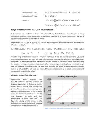
H=f(L/D)(U2/2g)
=>
dP/dx
=
(Delta
P)/(Delta
L)
=
fdarcy(Density)(U)2/2D
=
312.2
N/m^3
The
initial
conditions
(I.Cs)
and
boundary
conditions
(B.Cs)
are
highly
affecting
in
solution
process
of
the
numerical
methods.
If
we
consider
more
in
these
items,
we
will
have
easier
path
to
the
results.

3. For
inner
wall
r
=
ri
:
U
=
0,
T=Tw=cte=700+273.15
&
Z
=
-­‐(H*ri)
For
outer
wall
r
=
ro:
U
=
0,
dT/dr=0
For
x
=
0:
2𝜋𝑟! 𝜏! = 𝜋 ∗
!"
!"
∗ 𝑟!
!
− 𝑟!
!
→ 𝜏! = 4.34 𝑁/𝑚!
2𝜋𝑟! 𝜏! = 𝜋 ∗
!"
!"
∗ 𝑟!
!
− 𝑟!
!
→ 𝜏! = 3.79 𝑁/𝑚!
Runge-­‐Kutta
Method
with
MATLAB
in-­‐house
software:
In
this
section
we
would
like
to
describe
4th
order
of
Runge-­‐Kutta
technique
for
solving
the
ordinary
differential
equations.
Initial
values
need
to
be
chosen
carefully
in
all
numerical
methods.
The
set
of
equation
for
this
method
is
presented
as
below:
Regarded
to:
𝑦 = 𝑓(𝑥, 𝑦),
&
𝑦! = 𝑓(𝑥!),
we
use
4
auxiliary
points
and
therefore,
error
would
be
from
5th
order
(
…+O(h)5
):
𝑘! = ℎ𝑓(𝑥!, 𝑦!),𝑘! = ℎ𝑓(𝑥! + 1/2ℎ, 1/2𝑘!),𝑘! = ℎ𝑓(𝑥! + 1/2ℎ, 1/2𝑘!),𝑘! = ℎ𝑓(𝑥! + 1/2ℎ, 1/2𝑘!)
𝑥!!! = 𝑥! + ℎ,
&
𝑦!!! = 𝑦! + 1/6(𝑘! + 2𝑘! + 2𝑘! + 𝑘!),
4th
order
Rung-­‐Kutta
method
would
be
a
recursive
technique.
At
first
it
is
needed
to
initialize
T,
Z,
u
and
other
needed
constants,
and
then
it
is
required
to
construct
three
parallel
solvers
for
each
of
variables.
Using
MATLAB
we
can
easily
handle
the
iteration
process.
It
needs
to
update
the
values
after
calculating
the
weighted
averages.
Consequently,
calculating
for
4
functional
points
and
updating
variables
through
new
deltas
finalize
each
of
iterations.
The
main
point
would
be
that
with
x
increment
equation
variables
such
as
u,
Z,
T,
and
dT/dx
will
have
new
values.
This
procedure
contains
up
to
results
convergence
and
consequently
repetition
for
values.
Obtained
Results
from
MATLAB:
Optimization
results
obtained
from
MATLAB
software
presents
variation
of
targeted
parameters
in
following
figures.
Outlet
velocity
profile
and
steady-­‐state
profile
of
temperature
are
more
important.
Radius
variation
from
0.05
to
0.075
meter
shows
the
maximum
velocity
lower
than
60
m/s.
However,
for
outer
wall
final
temperature
is
lower
than
300o
C.
In
figure.3a
velocity
profile
shows
a
fully
turbulent
case
were
studied
and
very
low
velocity
values
next
to
wall
confirms
it.
0.05 0.06 0.07 0.08
-5000
-4000
-3000
-2000
-1000
0
1000
Z(w/m)
r(m)
Z=-Hþr
i
& H:heat flux
Figure
2:
Z
variation
regarded
to
inner
radius
and
Heat
Flux

4.
Part2:
Using
FLUENT
as
CFD
Software
The
main
concept
of
parallel
computing
with
FLUENT
relates
to
using
computational
fluid
dynamic
software.
Therefore,
we
can
compare
the
results
of
numerical
solution
with
RK4
via
MATLAB
and
with
ANSYS/FLUENT.
The
theory
of
the
problem
in
the
second
part
is
exactly
as
it
provided
with
the
first
part
and
consequently
we
can
define
the
same
results
from
simulated
model.
Boundary
conditions
and
initial
conditions
are
very
important
in
our
model,
and
steps
of
using
ANSYS/FLUENT
differ
with
In-­‐house
software.
The
following
steps
regularly
required
for
any
CFD
project
worked
with
ANSYS/FLUENT.
-­‐ Creating
the
geometry
2-­‐D
or
3-­‐D
(Using
Gambit
or
ANSYS
design
modeler)
-­‐ Determining
the
state
of
the
problem
(such
as
steady-­‐state
or
transient,
Newtonian,
compressibility,
…
)
-­‐ Applying
initial
conditions
on
relevant
walls,
inlets,
outlets,
symmetry
lines,
…
-­‐ Setting
needed
constants
and
defining
proper
values
for
them
-­‐ Using
appropriate
size
control
for
mesh
and
consequently
define
a
systematic
mesh
generator
-­‐ Define
a
calculation
method
and
algorithm
which
might
be
important
in
fluid
dynamic
cases
-­‐ Deriving
the
required
results
from
the
pool
of
solutions
Simply
this
project
enjoyed
a
k-­‐epsilon
turbulent
model
in
FLUENT
software.
And
directional
velocity
of
Ub=
50
m/s
launched
inside
the
pipes
between
ri=50 mm
&
ro=75 mm.
Results
of
temperature
profile
in
outlet
face
and
also
the
results
of
velocity
profile
after
fully-­‐developed
length
can
be
illustrated
in
figure4.
In
this
figure
we
can
find
that
there
would
be
a
viscous
sublayer
area
in
leass
than
5%
of
fluid
domain
from
each
wall
with
very
low
magnitude
for
the
velocity.
And
the
maximum
value
for
velocity
0 20 40 60
0.05
0.055
0.06
0.065
0.07
0.075
velocity(m/s)
r(m)
u-velocity profile
200 300 400 500 600 700
0.05
0.055
0.06
0.065
0.07
0.075
0.08
r(m)
T(° C)
Temperature profile
Figure
3a:
Velocity
profile
at
fully-­‐developed
level
of
annular
space
Figure
3b:
Temperature
profile
for
steady-­‐state
condition

5. hardly
reaches
to
60
m/s.
Again
as
it
is
obvious
from
the
boundary
conditions
we
have
dT/dx=0
at
the
outer
surface
and
the
minimum
temperature
of
460o
C
released
for
outer
wall
in
fully
developed
case.
Figure
4:
Results
of
temperature
profile
(right)
and
velocity
profile
(left)
by
FLUENT
plotted
against
various
radiuses.
Discussion:
There
would
be
various
problems
in
using
numerical
methods
in
engineering.
In
this
project
we
assumed
to
define
a
turbulence
fluid
for
inlet
air
and
consequently
the
other
constants
calculated
based
on
this
assumption.
We
also
selected
initial
values
for
U,
Z
and
T
for
launching
of
RK4
method.
We
know
that
efficiency
of
these
numerical
methods
highly
depends
on
estimating
true
initialization.
Some
sorts
of
similarities
can
be
easily
obvious
between
the
results
of
RK4
in
MATLAB
software
and
CFD
modelling
process
using
FLUENT.
Figure
5:
Grid
dependency
for
CFD
analysis
References:
1. F.
M.
White,
Fluid
Mechanics,
McGraw-­‐Hill.
2. http://Wikipedia.org/ODE45
3. ANSYS
CFX
Toturial
4. http://www.mbs-­‐europe.com/eng/webproduct.php?idarticolo=10
5. Project
Brief/
Professor
Wyszinsky,
University
of
Birmingham
6. Christie,
Ignas
S.
(Clay,
NY),
“Multi-­‐tube
heat
exchanger
with
annular
spaces”,
United
States
Patent
6626235,
Publication
Date:
09/30/2003
1.2 1.3 1.4 1.5 1.6 1.7 1.8
x
10
-­‐9
0.16
0.18
0.2
0.22
2D
cell
volume
Y-­‐pluse
grid
independency

6. Extra
task
(PART
III):
Investigate
flows
around
a
2-­‐d
circular
rod
immersed
in
flow
(using
ANSYS-­‐
FLUENT.)
Contents:
In
this
part
we
are
interested
to
investigate
the
effects
of
variation
in
Reynolds
number
in
stream
lines
and
flow
path
for
laminar
and
turbulent
flows.
For
this
purpose
a
2-­‐dimensional
circle
is
modeled
at
the
middle
of
a
plate
which
demonstrates
a
rod
immersed
in
various
types
of
flow.
The
aim
of
the
project
was
to
examine
the
type
of
flow,
wake,
velocity
profile,
and
path
of
stream
lines
against
different
number
of
Reynolds.
In
this
case
we
modeled
flow
with
7
different
Reynolds
numbers.
In
a
constant
geometry,
from
Re=1
to
Re=106
with
exponential
increment,
the
following
results
derived
in
figure6.
The
obtained
results
show
different
aspects
of
velocity
profile
in
outlet
wall
and
different
types
secondary
flows
and
vortices
in
upper
and
lower
walls
and
in
the
wake
space.
Generally,
from
the
velocity
profiles
at
the
outlet
we
can
easily
find
the
Re
number.
For
first
three
figures
there
are
smooth
and
parabolic
shape
for
velocity
profile
and
it
leads
to
laminar
flow
and
consequently
Newtonian
and
inviscid
fluid.
For
Re=1000
the
fluids
flows
in
laminar
model
but
neighboring
walls
affects
velocity
profile.
From
10000
to
1000000
we
can
see
that
viscous
sub-­‐layer
created
near
the
walls.
Viscous
sub-­‐layer
includes
less
than
5%
of
the
area
at
outlet
wall
or
totally
in
fully-­‐
developed
condition.
And
velocity
profile
approximately
takes
a
uniform
shape
in
middle
areas
of
outlet
wall.
One
of
the
main
points
which
is
completely
obvious
in
these
figures
can
be
mentioned
in
Re
number
between
1000
and
10000.
This
area
can
be
regarded
as
transition
between
laminar
and
turbulent
flows
which
contains
highest
amount
of
viscous
wake.
Separation
points
have
different
locations
circular
wall
and
it
completely
depends
on
Re
number.
Stagnation
points
at
the
start
and
end
of
circular
path
are
also
obvious
and
can
be
marginally