Inequality #4

Arthur CHARPENTIER - Welfare, Inequality and Poverty
Arthur Charpentier
charpentier.arthur@gmail.com
http://freakonometrics.hypotheses.org/
Université de Rennes 1, February 2016
Welfare, Inequality & Poverty, # 4
1

Regression?
Galton (1870, galton.org, 1886, galton.org ) and Pear-
son & Lee (1896, jstor.org, 1903 jstor.org) studied ge-
netic transmission of characterisitcs, e.g. the heigth.
On average the child of tall parents is taller than
other children, but less than his parents.
“I have called this peculiarity by the name of regres-
sion’, Francis Galton, 1886.
2

Regression?
1 > l i b r a r y ( HistData )
2 > attach ( Galton )
3 > Galton$ count <− 1
4 > df <− aggregate ( Galton , by=l i s t ( parent ,
c h i l d ) , FUN=sum) [ , c (1 ,2 ,5) ]
5 > plot ( df [ , 1 : 2 ] , cex=sqrt ( df [ , 3 ] / 3) )
6 > ab lin e ( a=0,b=1, l t y =2)
7 > ab lin e (lm( c h i l d ~parent , data=Galton ) )
q q q q q
q q q
q q q q q q q q
q q q q q q q
q q
q q
q q q q q
q q q q q q q q q
q q q q q q q q q
q
q q q q q q q q
q q q q q q q q q
q q q q q q q q
q q q q q q q
q q q q q q q q
q q q q q q
q q q q
64 66 68 70 72
62646668707274
height of the mid−parent
heightofthechild
q q q q q
q q q
q q q q q q q q
q q q q q q q
q q
q q
q q q q q
q q q q q q q q q
q q q q q q q q q
q
q q q q q q q q
q q q q q q q q q
q q q q q q q q
q q q q q q q
q q q q q q q q
q q q q q q
q q q q
3

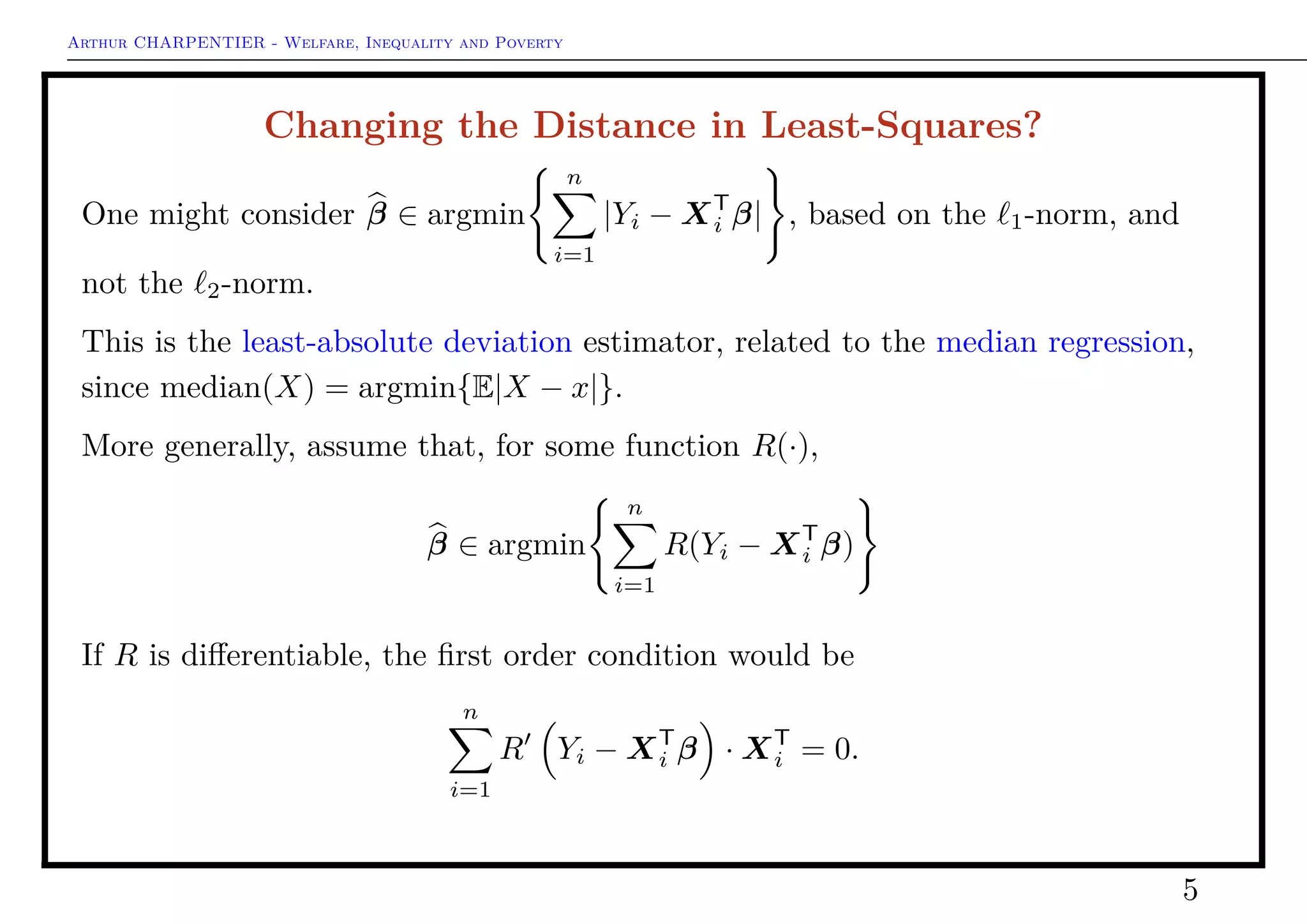
Least Squares?
Recall that



E(Y ) = argmin
m∈R
Y − m 2
2
= E [Y − m]2
Var(Y ) = min
m∈R
E [Y − m]2
= E [Y − E(Y )]2
The empirical version is



y = argmin
m∈R
n
i=1
1
n
[yi − m]2
s2
= min
m∈R
n
i=1
1
n
[yi − m]2
=
n
i=1
1
n
[yi − y]2
The conditional version is



E(Y |X) = argmin
ϕ:Rk→R
Y − ϕ(X) 2
2
= E [Y − ϕ(X)]2
Var(Y |X) = min
ϕ:Rk→R
E [Y − ϕ(X)]2
= E [Y − E(Y |X)]2
4

Changing the Distance in Least-Squares?
One might consider β ∈ argmin
n
i=1
|Yi − XT
i β| , based on the 1-norm, and
not the 2-norm.
This is the least-absolute deviation estimator, related to the median regression,
since median(X) = argmin{E|X − x|}.
More generally, assume that, for some function R(·),
β ∈ argmin
n
i=1
R(Yi − XT
i β)
If R is diﬀerentiable, the ﬁrst order condition would be
n
i=1
R Yi − XT
i β · XT
i = 0.
5

i.e.
n
i=1
ω Yi − XT
i β
ωi
· Yi − XT
i β XT
i = 0 with ω(x) =
R (x)
x
,
It is the ﬁrst order condition of a weighted 2 regression.
To obtain the 1-regression, observe that ω = |ε|−1
6

=⇒ use iterative (weighted) least-square regressions.
Start with some standard 2 regression
1 > reg_0 <− lm(Y~X, data=db)
For the 1 regression consider weight function
1 > omega <− function ( e ) 1/abs ( e )
Then consider the following iterative algorithm
1 > r e s i d <− r e s i d u a l s ( reg_0)
2 > f o r ( i in 1:100) {
3 + W <− omega ( e )
4 + reg <− lm(Y~X, data=db , weights=W)
5 + e <− r e s i d u a l t s ( reg ) }
q
q
q
q
q
q
q
q
q
q
q
q
q
q
q
q
qq
q
q
q
q
q
q
q
q
q
q
q
q
q
q
q
q
q
q
q
q
q
q
q
q
q
q
q
q
qq
q
q
speed
dist
5 10 15 20 25
020406080100120
7

Quantile Regression
Observe that, for all τ ∈ (0, 1)
QX(τ) = F−1
X (τ) = argmin
m∈R
{E[Rτ (X − m)]}
where Rτ (x) = [τ − 1(x < 0)] · x.
From a statistical point of view
Qx(τ) = argmin
m∈R
1
n
n
i=1
Rτ (xi − m) .
The quantile-τ regression
β = argmin
n
i=1
Rτ (Yi − XT
i β) .
8

q
5 10 15 20 25
020406080100120
speed
dist
q
q
q
5 10 15 20 25
020406080100120
speed
dist
5 10 15 20 25
020406080100120
speed
dist
There are n(1 − p) points in the upper region, and np in the lower one.
1 > l i b r a r y ( quantreg )
2 > f i t 1 <− rq ( y ~ x1 + x2 , tau = . 1 , data = df )
see cran.r-project.org.
9

Quantile Regression: Empirical Analysis
Consider here some salaries, as a func-
tion of the experience (in years), see
data.princeton.edu
1 > s a l a r y=read . table ( " http : // data .
princeton . edu/wws509/ datasets
/ s a l a r y . dat " , header=TRUE)
2 > l i b r a r y ( quantreg )
3 > plot ( s a l a r y $yd , c )
4 > ab lin e ( rq ( s l ~yd , tau =.1 , data=
s a l a r y ) , c o l=" red " )
q
q
q
q
q
q
q
q q
q
q
q
q
q
q
q
q
q
q
q
q
q
q
q
q
q
q
q
q
q
q
q
q
q
q
q
q
q
q
q
q q
q
q
q
q q
q
q
q
q
q
0 5 10 15 20 25 30 35
1500020000250003000035000
Experience (years)
Salary
10

1 > u <− seq ( . 0 5 , . 9 5 , by=.01)
2 > c o e f s t d <− function (u) summary(
rq ( s l ~yd , data=salary , tau=u) ) $
c o e f f i c i e n t s [ , 2 ]
3 > c o e f e s t <− function (u) summary(
rq ( s l ~yd , data=salary , tau=u) ) $
c o e f f i c i e n t s [ , 1 ]
4 > CS <− Vectorize ( c o e f s t d ) (u)
5 > CE <− Vectorize ( c o e f e s t ) (u)
6 > CEinf <− CE−2∗CS
7 > CEsup <− CE+2∗CS
8 > plot (u ,CE[ 2 , ] , ylim=c ( −500 ,2000)
, c o l=" red " )
9 > polygon ( c (u , rev (u) ) , c ( CEinf
[ 2 , ] , rev (CEsup [ 2 , ] ) ) , c o l="
yellow " , border=NA)
qqqqqqq
qqqqqqqqqqq
qqqqqqq
q
qqqqqqqqqq
qqqqqqq
qqqqqqqqqqqqqqqqqq
qqqqqqqqqqqqqq
qqqq
qq
qqq
qqqqqqq
0.2 0.4 0.6 0.8
−5000500100015002000
probability
CE[2,]
11

Consider the evolution of the 90%−10%
quantile ratio,
1 > ratio9010 = function ( age ) {
2 + p r e d i c t (Q90 , newdata=data .
frame ( yd=age ) ) /
3 + p r e d i c t (Q10 , newdata=data .
frame ( yd=age ) )
4 + }
5 > ratio9010 (5)
6 1.401749
7 > A=0:30
8 > plot (A, Vectorize ( ratio9010 ) (A) ,
type=" l " , ylab=" 90−10 qua nti le
r a t i o " )
12

Local Regression: Empirical Analysis
which is smoother than the local esti-
mator
1 > ratio9010_k = function ( age , k
=10){
2 + idx=which ( rank ( abs ( s a l a r y $yd−
age ) )<=k)
3 + qu antil e ( s a l a r y $ s l [ idx ] , . 9 ) /
qu a ntile ( s a l a r y $ s l [ idx ] , . 1 ) }
4 > A=0:30
5 > plot (A, Vectorize ( ratio9010_k) (A
) , type=" l " , ylab=" 90−10
qu a ntile r a t i o " )
13

Local Regression: Empirical Analysis
1 > Gini ( s a l a r y $ s l )
2 [ 1 ] 0.1391865
We can also consider some local Gini
index
1 > Gini_k = function ( age , k=10){
2 + idx=which ( rank ( abs ( s a l a r y $yd−
age ) )<=k)
3 + Gini ( s a l a r y $ s l [ idx ] ) }
4 > A=0:30
5 > plot (A, Vectorize ( Gini_k ) (A) ,
type=" l " , ylab=" Local Gini
index " )
14

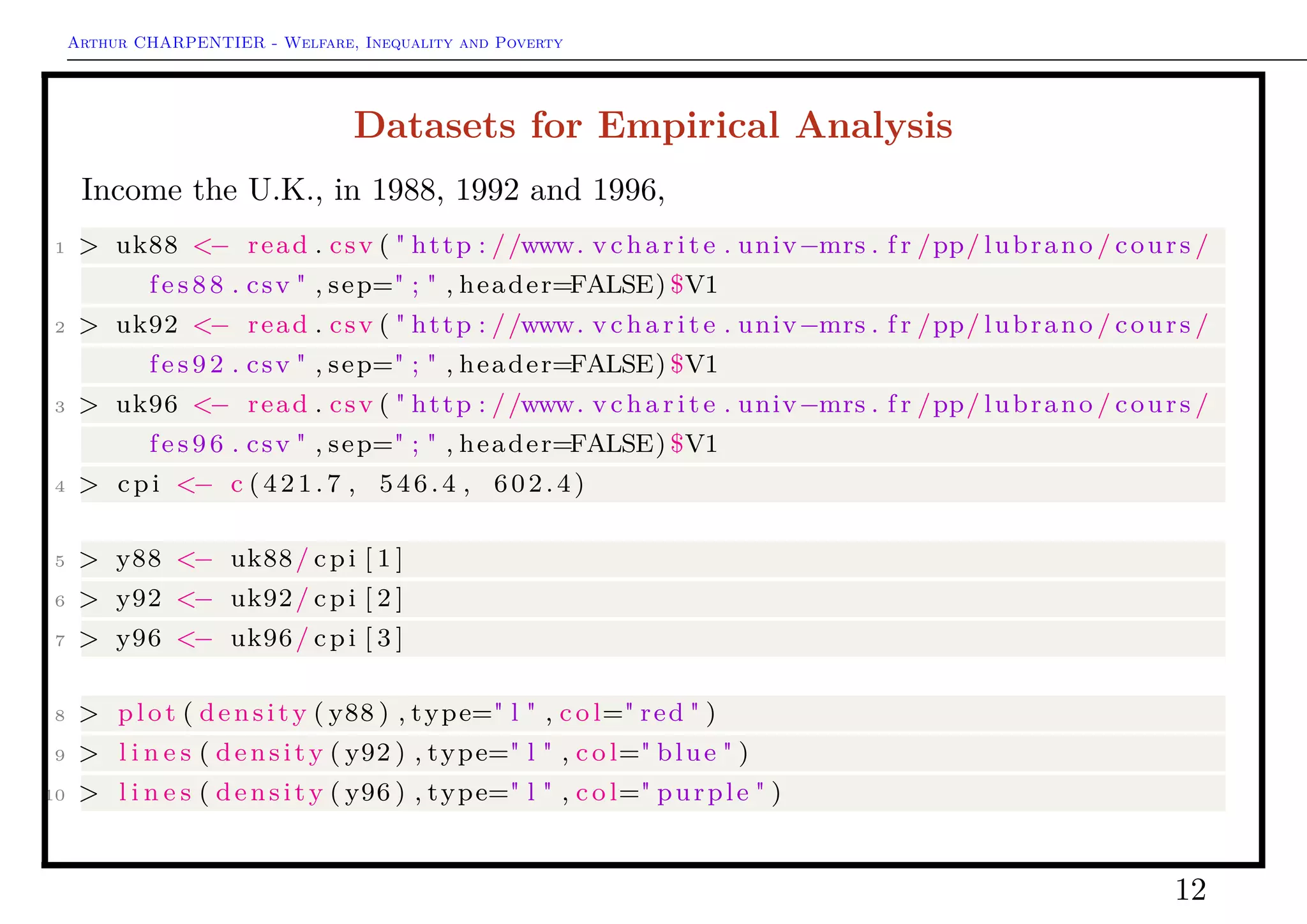
Datasets for Empirical Analysis
Income the U.K., in 1988, 1992 and 1996,
1 > uk88 <− read . csv ( " http : //www. v char it e . univ−mrs . f r /pp/ lubrano / cours /
f e s 8 8 . csv " , sep=" ; " , header=FALSE) $V1
4 > cpi <− c (421.7 , 546.4 , 602.4)
5 > y88 <− uk88/ cpi [ 1 ]
6 > y92 <− uk92/ cpi [ 2 ]
7 > y96 <− uk96/ cpi [ 3 ]
8 > plot ( density ( y88 ) , type=" l " , c o l=" red " )
9 > l i n e s ( density ( y92 ) , type=" l " , c o l=" blue " )
10 > l i n e s ( density ( y96 ) , type=" l " , c o l=" purple " )
15

Datasets for Empirical Analysis
16

Inequalities: Empirical Analysis
We can visualize empirical Lorenz curves, and theoretical version (lognormal)
1 > plot ( Lc ( y88 ) ) ; s=sd ( log ( y88 ) ) ; l i n e s ( Lc . lognorm , parameter=s )
17

If we plot the three curves on the same
graph,
1 > plot ( Lc ( y88 ) , c o l=" red " )
2 > l i n e s ( Lc ( y92 ) , c o l=" blue " )
3 > l i n e s ( Lc ( y96 ) , c o l=" purple " )
18

1 > i n e q u a l i t i e s=function ( f_ineq ) {
2 + z88 =f_ineq ( y88 ) ; z92 = f_ineq
( y92 ) ; z96 = f_ineq ( y96 )
3 + I=cbind ( z88 , z92 , z96 )
4 + names ( I )=c ( " 1988 " , " 1992 " , " 1996
" )
5 + cat ( " 1 9 8 8 . . . " , z88 , " n 1 9 9 2 . . .
" , z92 , " n 1 9 9 6 . . . " , z96 , " n" )
6 + barplot ( I , c o l=" l i g h t green " ,
names . arg=c ( " 1988 " , " 1992 " , "
1996 " ) )
7 + return ( I ) }
8 > I<−i n e q u a l i t i e s ( Gini )
9 1 9 8 8 . . . 0.3073511
10 1 9 9 2 . . . 0.3214023
11 1 9 9 6 . . . 0.2975789
19

1 > I<−i n e q u a l i t i e s ( Theil )
2 1 9 8 8 . . . 0.1618547
3 1 9 9 2 . . . 0.1794008
4 1 9 9 6 . . . 0.1506973
20

Welfare Functions
A welfare function as a function with n arguments W(x) = W(x1, · · · , xn).
Assume that W is normalize, so that W(1) = 1.
It represents social preferences over the income distribution, and it should satisfy
some axioms,
Pareto axiom: The welfare function is increasing for all its inputs
W(x + ) ≥ W(x) for all ≥ 0.
Symmetry axiom or anonymity: We can permute the individuals without
changing the value of the function
W(x1, x2, · · · , xn) = W(x2, x1, · · · , xn)
21

Welfare Functions
Principle of transfers: the quasi concavity of the welfare function implies that if
we operate a monetary transfer from a rich to a poor, welfare is increased,
provided that the transfer does not modify the ordering of individuals
(Pigou-Dalton principle)
W(x1, · · · , xi, · · · , xj, · · · , xn) ≥ W(x1, · · · , xi+δ, · · · , xj−δ, · · · , xn)
Other axioms can be added, e.g. homogeneous of order 1,
W(λx) = λW(x) for all λ ≥ 0.
Thus (all homogeneous function of order 1 can be deﬁned on the simplex)
W(x) = x · W
x
x
for all λ ≥ 0.
22

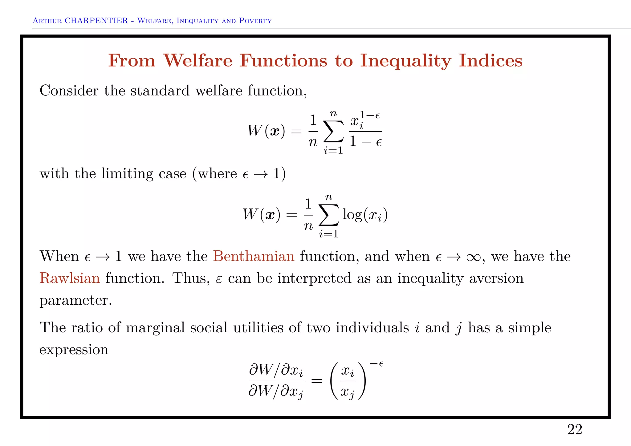
Welfare Functions
Observe that W(x1) = x. And because of the aversion for inequality, W(x) ≤ x.
One can denote
W(x) = x · [1 − I(x)]
for some function I(·), which takes values in [0, 1].
I(·) is then interpreted as an inequality measure and x · I(x) represents the
(social) cost of inequality.
See fao.org.
23

Welfare Functions
E.g. utilitarian (or Benthamian) function
W(x) = x =
1
n
n
i=1
xi
“dollar is a dollar” approach: no inequality aversion.
E.g. Rawlsian welfare function
W(x) = min{y1, · · · , yn}.
Social welfare cannot increase unless the income of the poorest individual is
increased: inﬁnite inequality aversion.
24

From Welfare Functions to Inequality Indices
Consider the standard welfare function,
W(x) =
1
n
n
i=1
x1−
i
1 −
with the limiting case (where → 1)
W(x) =
1
n
n
i=1
log(xi)
When → 1 we have the Benthamian function, and when → ∞, we have the
Rawlsian function. Thus, ε can be interpreted as an inequality aversion
parameter.
The ratio of marginal social utilities of two individuals i and j has a simple
expression
∂W/∂xi
∂W/∂xj
=
xi
xj
−
25

When increases, the marginal utility of the poorest dominates, see Rawls (1971)
wikipedia.org, the objective of the society is to maximise the situation of the
poorest.
From that welfare function, deﬁne the implied inequality index,
I = 1 −
1
n
n
i=1
xi
x
1−
1
1−ε
which is Atkinson index.
26

Equally Distributed Equivalent
Given x define ξ (or ξ(x)) as
W(ξ1) = W(x)
From the principle of transfers, ξ ≤ x. Then one can define
I(x) = 1 −
ξ(x)
x
.
If I(·) satisfies the scale independence axiom, I(x) = I(λx), then
ξ(x) =
1
n
n
i=1
(xi)
1−
1
1−ε
This index has a simple interpretation : if I = 0.370% of the total income is
necessary to reach the same value of welfare, provided that income is equally
distributed.
27

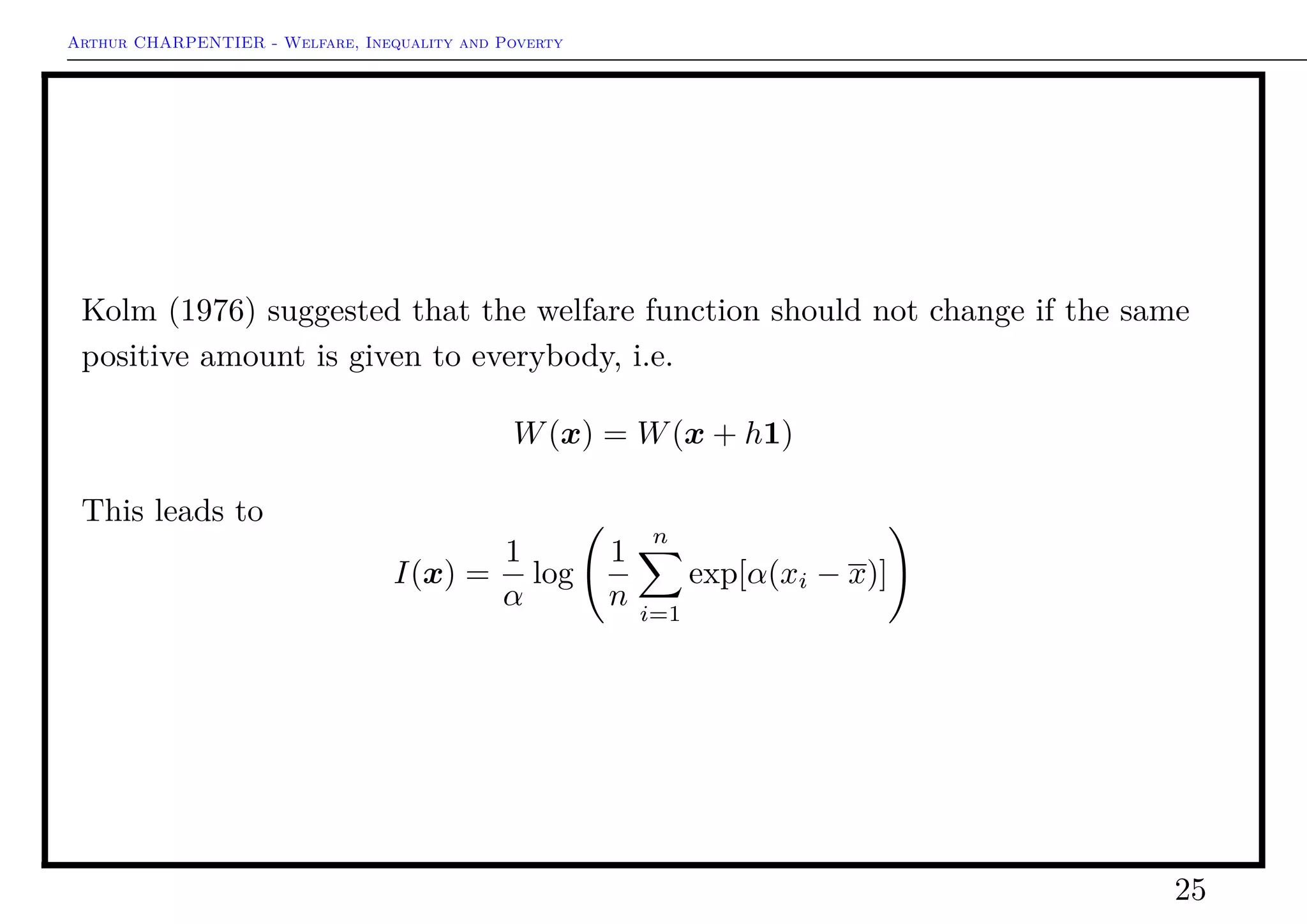
Kolm (1976) suggested that the welfare function should not change if the same
positive amount is given to everybody, i.e.
W(x) = W(x + h1)
This leads to
I(x) =
1
α
log
1
n
n
i=1
exp[α(xi − x)]
28

From Inequality Indices to Welfare Functions
Consider e.g. Gini index
G(x) =
2
n(n − 1)x
n
i=1
i · xi:n −
n + 1
n − 1
G(x) =
1
2n2x
n
i,j=1
|xi − xj|
then deﬁne
W(x) = x · [1 − G(x)]
as suggested in Sen (1976, jstor.org)
More generally, consider
W(x) = x · [1 − G(x)]σ
with σ ∈ [0, 1].
29

From Inequality to Poverty
an absolute line of poverty is defined with respect to a minimum level of
subsistence
In developed countries and more precisely within the EU, o ne prefer to define a
relative poverty line, defined with respect to a fraction of the mean or the median
of the income distribution.
The headcount ratio evaluates the number of poor (below a threshold z)
H(x, z) =
1
n
n
i=1
1(xi ≤ z) = F(z) =
q
n
where q is the number of poors.
The income gap ratio I(x, z) measures in percentage the gap between the poverty
line z and the mean income among the poor
I(x, z) =
1
z
z −
1
q
n
i=1
xi1(xi ≤ z) =
1
z
z −
1
q
q
i=1
xi:n = 1 −
µp
z
30

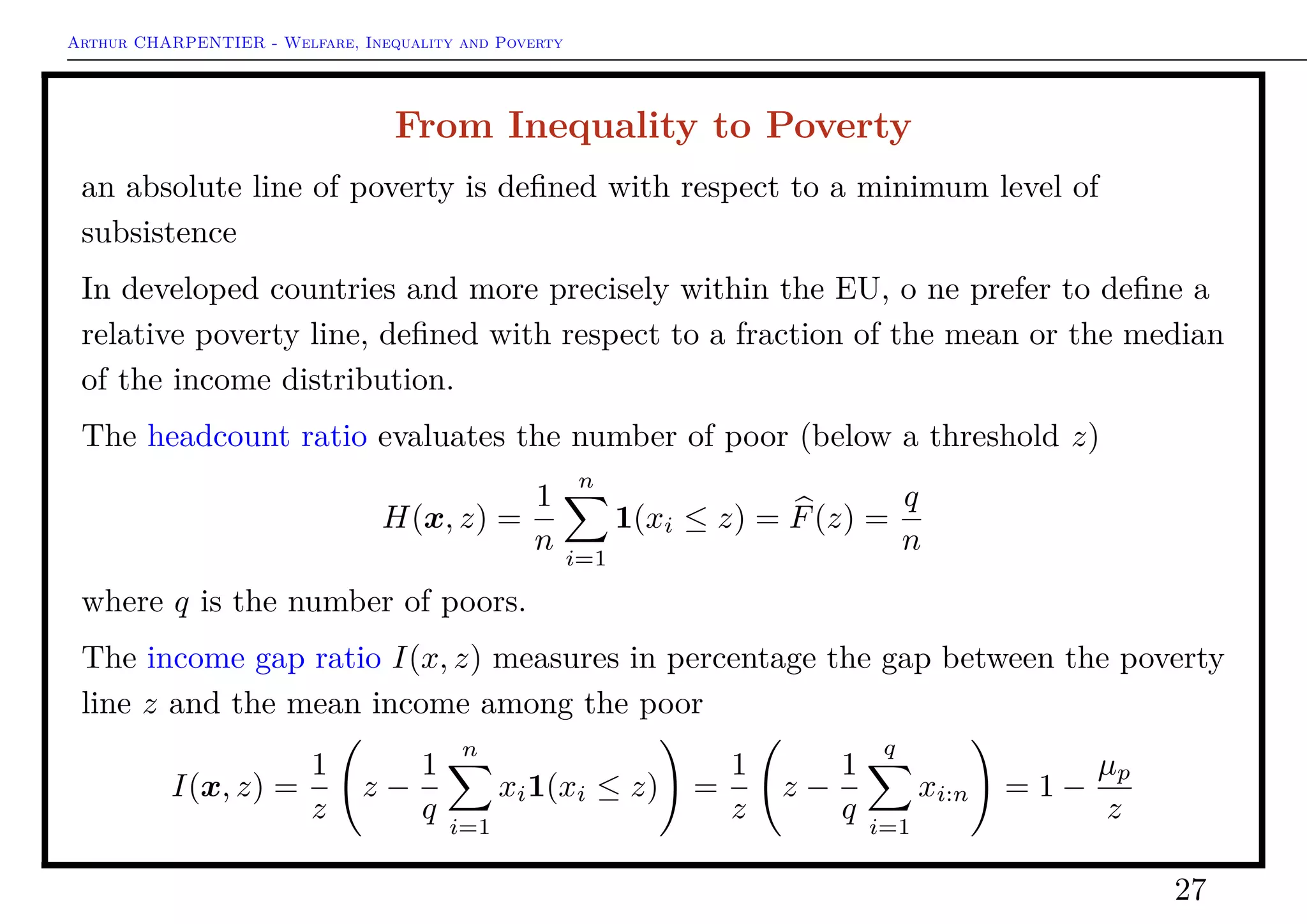
where µp is the average income of the poor.
The poverty gap ratio is deﬁned as
HI(x, z) =
q
n
1 −
1
qz
q
i=1
xi:n
Watts (1968) suggested also
W(x, z) =
1
q
q
i=1
[log z − log xi:n]
which can be writen
W = H · (T − log(1 − I))
where T is Theil index (Generalize Entropy, with index 1)
T =
1
n
n
i=1
xi
x
log
xi
x
.
1 > Watts (x , z , na . rm = TRUE)
31

Sen Poverty Indices
S(x, z) = H(x, z) · [I(x, z) + [1 − (x, z)]Gp]
where Gp is Gini index of the poors.
• if Gp = 0 then S = HI
• if Gp = 1 then S = H
1 > Sen (x , z , na . rm = TRUE)
On can write
S =
2
(q + 1)nz
q
i=1
[z − xi:n][q + 1 − i]
Thon (1979) suggested a similar expression, but with (slightly) diﬀerent weights
Thon =
2
n(n + 1)z
q
i=1
[z − xi:n][n + 1 − i]
32

But it suﬀers some drawbacks: it violates the principle of transfers and is not
continuous in x. Shorrocks (1995, jstor.org) suggested
SST(x, z) = [2 − H(x, z)] · H(x, z) · I(x, z) + H(x, z)2
[1 − I(x, z)] · GP
Observe that Sen index is deﬁned as
S =
2
(q + 1)n
q
i=1
z − xi:n
z
˜xi
[q + 1 − i]
while
SST =
1
n2
q
i=1
z − xi:n
z
˜xi
[2n − 2i + 1]
This index is symmetric, monotonic, homogeneous of order 0 and takes values in
[0, 1]. Further it is continuous and consistent with the transfert axiom.
On can write
SST = ˜x · [1 − G(˜x)].
33

1 > SST(x , z , na . rm = TRUE)
1 > poverty=function ( f_pov , z_fun=function (x ) mean( x ) / 2 , . . . ) {
2 + z88 =z_fun ( y88 ) ; z92 = z_fun ( y92 ) ; z96 = z_fun ( y96 )
3 + p88=f_pov ( y88 , z88 ) ; p92=f_pov ( y92 , z92 ) ; p96=f_pov ( y96 , z96 )
4 + P=cbind ( p88 , p92 , p96 )
5 + names (P)=c ( " 1988 " , " 1992 " , " 1996 " )
6 + cat ( " 1 9 8 8 . . . " , p88 , " n 1 9 9 2 . . . " , p92 , " n 1 9 9 6 . . . " , p96 , " n" )
7 + barplot (P, c o l=" l i g h t green " , names . arg=c ( " 1988 " , " 1992 " , " 1996 " ) )
8 + return (P) }
34

FGT Poverty Indices
Foster, Greer & Thorbecke (1984, darp.lse.ac.uk) suggested a class of poverty
indices that were decomposable,
Pα(x, z) =
1
n
q
i=1
1 −
xi
z
α
where α ∈ {0, 1, 2, · · · }.
When α = 0 we get the headcount measure,
P0 =
1
n
q
i=1
1(xi ≤ z) =
q
n
When α = 1 we get an average of poverty gap z − xi
P1 =
1
n
q
i=1
1 −
xi
z
1(xi ≤ z)
35

(see HI).
In R, the parameter is 1 + α
1 > Foster (x , k , parameter = 1 , na . rm = TRUE)
i.e. it gives for parameter 1 the headcount ratio and for parameter 2 the poverty
gap ratio.
When α = 2
P2 =
1
n
q
i=1
1 −
xi
z
2
1(xi ≤ z)
36

1 > P<−poverty ( Watts , function ( x)
mean(x ) / 2)
2 1 9 8 8 . . . 0.03561864
3 1 9 9 2 . . . 0.05240638
4 1 9 9 6 . . . 0.03342492
1 > P<−poverty ( Watts , function ( x)
qu a ntile (x , . 1 ) )
2 1 9 8 8 . . . 0.01935494
3 1 9 9 2 . . . 0.0277594
4 1 9 9 6 . . . 0.02289631
37

1 > P<−poverty ( Sen , function ( x) mean
( x ) / 2)
2 1 9 8 8 . . . 0.04100178
3 1 9 9 2 . . . 0.05507059
4 1 9 9 6 . . . 0.03640762
1 > P<−poverty ( Foster , function (x )
mean(x ) / 2 , param=0)
2 1 9 8 8 . . . 0.1714684
3 1 9 9 2 . . . 0.1925117
4 1 9 9 6 . . . 0.1421479
38

Group Decomposabilty
Assume that x is either x1 with probability p (e.g. urban) or x2 with probability
1 − p (e.g. rural). The (total) FGT index can be writen
Pα = p ·
1
n i,1
1 −
xi
z
α
+ [1 − p] ·
1
n i,2
1 −
xi
z
α
= pP(1)
α + [1 − p]P(2)
α
39

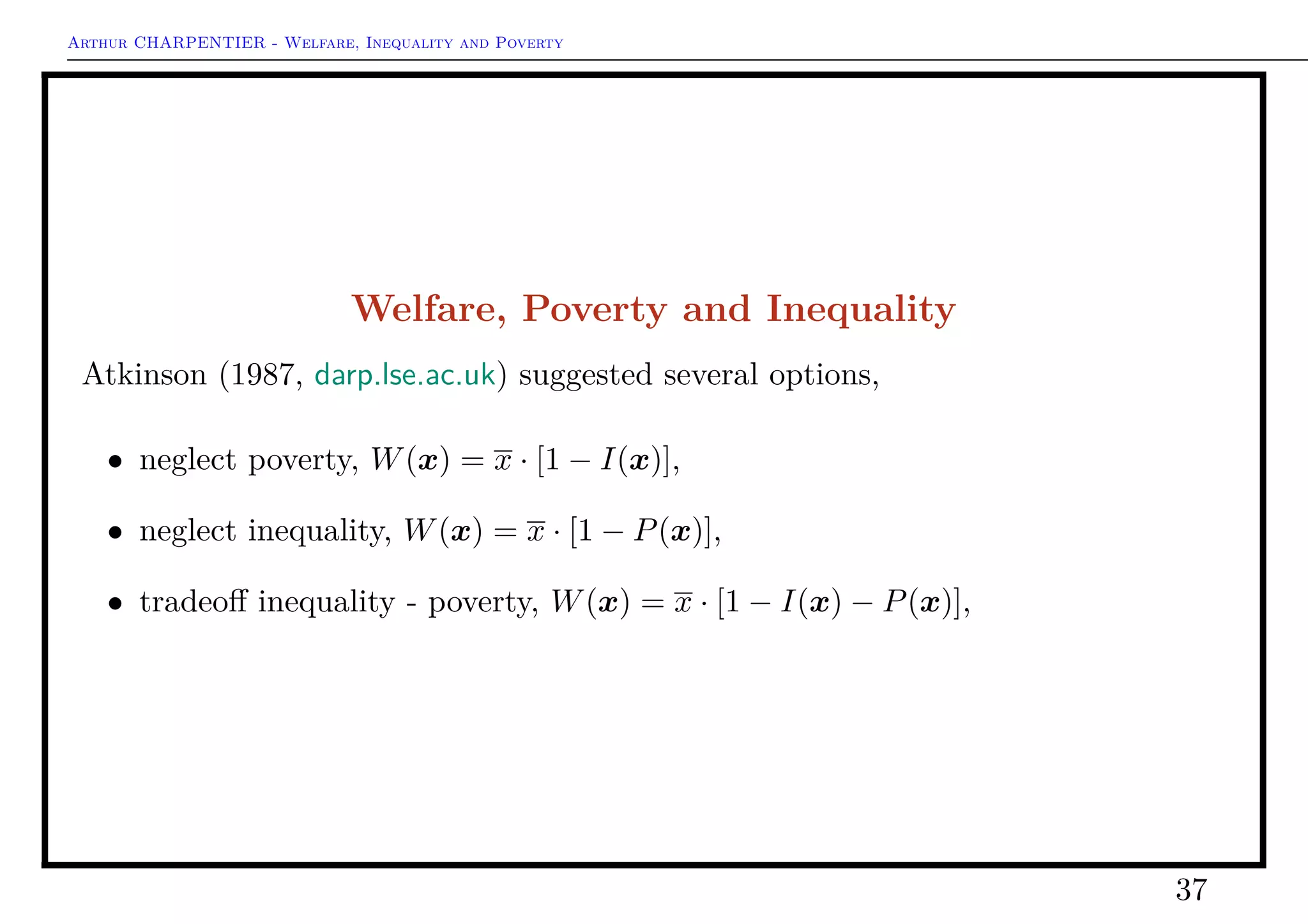
Welfare, Poverty and Inequality
Atkinson (1987, darp.lse.ac.uk) suggested several options,
• neglect poverty, W(x) = x · [1 − I(x)],
• neglect inequality, W(x) = x · [1 − P(x)],
• tradeoﬀ inequality - poverty, W(x) = x · [1 − I(x) − P(x)],
40

Projects
• Une réduction de l’inégalité des chances dans l’obtention du revenu en France
? pdf, 2004
• Socioeconomic inequalities in health: Measurement, computation and
statistical inference pdf, 1997
• Gini ou Entropie pdf, 2003
41

Inequality #4

More Related Content

What's hot

Viewers also liked

Similar to Inequality #4

More from Arthur Charpentier

Recently uploaded

Inequality #4