Downloaded 26 times


![Arthur CHARPENTIER - Actuariat de l’Assurance Non-Vie, # 8
Les trois lois limites
Ces trois lois sont en fait les trois cas particulier de la distribution GEV -
Generalized Extreme Value (représentation de Jenkinson-von Mises)
H (x) =
exp − [1 − ξ (x − µ) /σ]
1/ξ
si ξ = 0
exp (− exp [− (x − µ) /σ]) si ξ = 0
dès lors que µ + ξx/σ > 0.
Remarque S’il existe des constantes de normalisation an ∈ R et bn > 0, et une
loi non-dégénérée GEV(ξ) telles que
b−1
n {Xn:n − an}
L
→ GEV(ξ).
on dira que FX appartient au max-domain d’attraction (MDA) de GEV(ξ).
@freakonometrics 4](https://image.slidesharecdn.com/slides-ensae-2016-8-161119144952/75/Slides-ensae-2016-8-4-2048.jpg)
![Arthur CHARPENTIER - Actuariat de l’Assurance Non-Vie, # 8
Les grands risques
On peut définir des risques sous-exponentiels, si Xi est une suite de variables i.i.d.
lim
x→∞
P [X1 + ... + Xn > x]
P [max {X1, ..., Xn} > x]
= 1, n ≥ 1.
Définition Si FX est une fonction de répartition continue d’espérance E [X], on
définit l’indice de grands risques par
DFX
(p) =
1
E [X]
1
1−p
F−1
X (t) dt pour p ∈ [0, 1] .
La version empirique est alors Tn (p) la proportion des [np] plus gros sinistres par
rapport à la somme totale, i.e.
Dn (p) =
X1:n + X2:n + ... + X[np]:n
X1 + ... + Xn
où
1
n
< p ≤ 1.
@freakonometrics 5](https://image.slidesharecdn.com/slides-ensae-2016-8-161119144952/75/Slides-ensae-2016-8-5-2048.jpg)

![Arthur CHARPENTIER - Actuariat de l’Assurance Non-Vie, # 8
Loi de type Pareto
La loi de X est à variation régulière d’indice α ∈ (0, +∞) si pour tout x
lim
t→∞
P[X > tx]
P[X > t]
= lim
t→∞
F(tx)
F(t)
= x−α
ou encore
P[X > x] = x−α
L(x) où L est à variation lente, i.e. lim
t→∞
L(tx)
L(t)
= 1.
@freakonometrics 8](https://image.slidesharecdn.com/slides-ensae-2016-8-161119144952/75/Slides-ensae-2016-8-8-2048.jpg)

![Arthur CHARPENTIER - Actuariat de l’Assurance Non-Vie, # 8
Quelques estimateurs classiques de ξ
ξP ickands
n,k =
1
log 2
log
Xn−k:n − Xn−2k:n
Xn−2k:n − Xn−4k:n
ξHill
n,k =
1
k
k
i=1
log Xn−i:n − log Xn−k+1:n
ξDEdH
n,k = ξ
H(1)
n,k + 1 −
1
2
1 −
ξ
H(1)
n,k
2
ξ
H(2)
n,k
−1
,
où
ξ
H(r)
n,k =
1
k
k−1
i=1
[log Xn−i:n − log Xn−k:n]
r
, r = 1, 2, ..
@freakonometrics 10](https://image.slidesharecdn.com/slides-ensae-2016-8-161119144952/75/Slides-ensae-2016-8-10-2048.jpg)


![Arthur CHARPENTIER - Actuariat de l’Assurance Non-Vie, # 8
Estimation de quantiles extrêmes
Le quantile d’ordre p ∈]0, 1[ - correspondant à la Value-at-Risk - associé à X, de
fonction de répartition FX, se définie par
V aR(X, p) = xp = F−1
(p) = sup{x ∈ R, F(x) ≥ p}.
Notons que les assureurs parle plutôt de période de retour. Si T est la première
année où on observe un phénomène qui se produit annuellement avec probabilité
p. Alors
P[T = k] = [1 − p]k−1
p de telle sorte que E[T] =
1
p
Parmi les autres mesures pertinantes (et intéressantes en réassurance), on
retiendra la TV aR - ou ES - correspondant à la valeur moyenne sachant que la
V aR a été dépassée,
TV aR(X, p) = E(X|X > V aR(X, p)).
@freakonometrics 15](https://image.slidesharecdn.com/slides-ensae-2016-8-161119144952/75/Slides-ensae-2016-8-15-2048.jpg)


![Arthur CHARPENTIER - Actuariat de l’Assurance Non-Vie, # 8
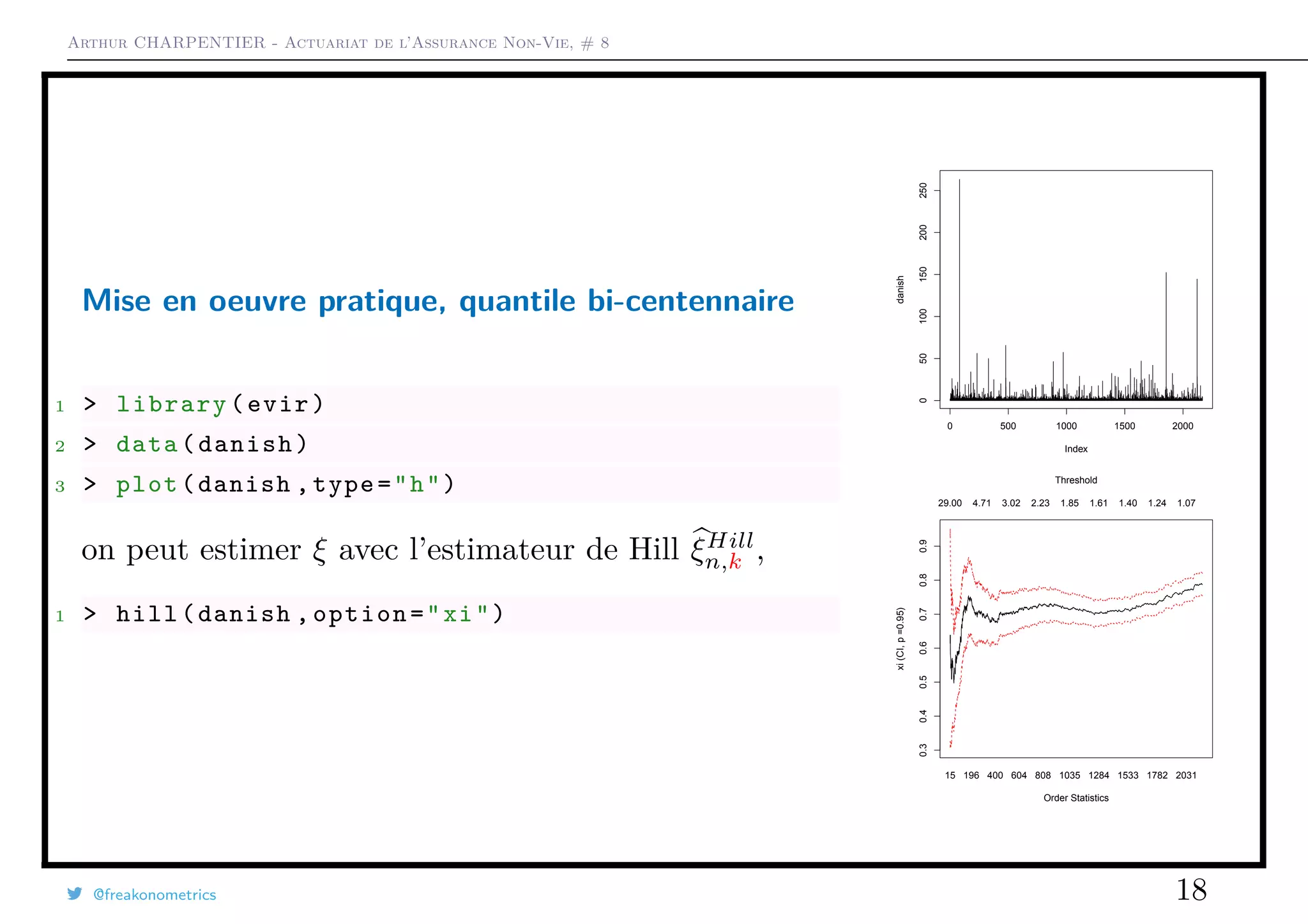
Mise en oeuvre pratique, quantile bi-centennaire
La densité de la loi de Pareto, en fonction de ξ et σ est
gξ,σ(x) =
1
σ
1 +
ξx
σ
− 1
ξ −1
que l’on peut écrire en fonction de ξ et Qp, si on considère une loi de Pareto au
delà d’un seuil u,
gξ,Qp
(x) =
n
Nu
(1 − p)
−ξ
− 1
ξ[Qp − u]
1 +
n
Nu
(1 − p)
−ξ
− 1
[Qp − u]
· x
− 1
ξ −1
1 > gq=function(x,xi ,q){
2 + ( (n/nu*(1-p) )^(-xi) -1)/(xi*(q-u))*(1+((n/nu*(1-p))^(-xi) -1)/(q-u)
*x)^(-1/xi -1)}
@freakonometrics 21](https://image.slidesharecdn.com/slides-ensae-2016-8-161119144952/75/Slides-ensae-2016-8-21-2048.jpg)
![Arthur CHARPENTIER - Actuariat de l’Assurance Non-Vie, # 8
Mise en oeuvre pratique, quantile bi-centennaire
On cherche le maximum de vraisemblance
(ξ, Qp) = argmax
Nu−1
i=0
log[gξ,Qp
(xn−i:n)]
log[L(ξ,Qp)]
1 > loglik=function(param){
2 + xi=param [2];q=param [1]
3 + lg=function(i) log(gq(Xs[i],xi ,q))
4 + return(-sum(Vectorize(lg)(1: nu)))}
50 100 150 200
0.20.40.60.81.0
Q
XI
−920
−930
−950
−975
−975
−1000
−1000
−1500
@freakonometrics 22](https://image.slidesharecdn.com/slides-ensae-2016-8-161119144952/75/Slides-ensae-2016-8-22-2048.jpg)
![Arthur CHARPENTIER - Actuariat de l’Assurance Non-Vie, # 8
Mise en oeuvre pratique, quantile bi-centennaire
ou mieux, le maximum de la vraisemblance profilée (seul Qp nous intéresse),
Qp = argmax max
ξ
{log[L(ξ, Qp)]}
1 > PL=function(Q){
2 + profilelikelihood =function(xi){
3 + loglik(c(Q,xi))}
4 + return(optim(par =.6,fn= profilelikelihood )$
value)} 30 40 50 60 70 80 90 100
−960−950−940−930−920
99.5% quantile
ProfileLikelihood
1 > (OPT=optimize(f=PL ,interval=c(10 ,100)))
2 $minimum
3 [1] 51.42182
4
5 $objective
6 [1] 918.2469
@freakonometrics 23](https://image.slidesharecdn.com/slides-ensae-2016-8-161119144952/75/Slides-ensae-2016-8-23-2048.jpg)
![Arthur CHARPENTIER - Actuariat de l’Assurance Non-Vie, # 8
Mise en oeuvre pratique, quantile bi-centennaire
On peut utiliser le test de rapport de vraisemblance pour obtenir un intervalle de
confiance, puisque
2 log[Lp(Qp)] − log[Lp(Qp)]
L
→ χ2
(1), lorsque n → ∞.
1 > XQ=seq (30 ,100 , length =101)
2 > L=Vectorize(PL)(XQ)
3 > up=OPT$objective
4 > I=which(-L>=-up -qchisq(p=.95 ,df=1)/2)
5 > range(XQ[I])
6 [1] 45.4 60.1
On peut utiliser le code suivant
1 > gpd.q(tailplot(gpd(Xs ,u)) ,.995)
qqqqqqqqqqqqqqqqqqqqqqqqqqqqqqqqqqqqqqqqqqqqqqqqqqqqqqqqqqqqqqqqqqqqqqqqqqqqqqqqqqqqqqqqqqqqqqqqqqqqqqqqqqqqqqqqqqqqqqqqqqqqqqqqqqqqqqqqqqqqqqqqqqqqqqqqqqqqqqqqqqqqqqqqqqqqqqqqqqqqqqqqqqqqqqqqqqqqqqqqqqqqqqqqqqqqqqqqqqqqqqqqqqqqqqqqqqqqqqqqqqq
q
q
q
q
q
q
q
q
q
q
q
5 10 20 50 100 200
2e−041e−035e−032e−021e−01
x (on log scale)
1−F(x)(onlogscale)
9995
@freakonometrics 24](https://image.slidesharecdn.com/slides-ensae-2016-8-161119144952/75/Slides-ensae-2016-8-24-2048.jpg)
![Arthur CHARPENTIER - Actuariat de l’Assurance Non-Vie, # 8
Choix du seuil u
Supposons que l’on choisisse un seuil u tel que u = Xn−k:n, alors
xp,k = Xn−k:n +
βk
ξk
n
k
(1 − p)
−ξk
− 1 ,
pour k > n(1 − p). On notera que si k = n(1 − p), xp,k coïncide avec l’estimateur
empirique du quantile, i.e. X[np+1]:n. Notons de plus que
MSE(xp) = V ar(xp) + E(xp − V aR(X, p))2
.
@freakonometrics 25](https://image.slidesharecdn.com/slides-ensae-2016-8-161119144952/75/Slides-ensae-2016-8-25-2048.jpg)
![Arthur CHARPENTIER - Actuariat de l’Assurance Non-Vie, # 8
Estimation de la période de retour
Pour rappel, le niveau Pm période de retour associée à une période de m années
(niveau qui sera excédé, en moyenne, toutes les m observations) est la solution de
P(X > u) 1 + ξ
Pm − u
σ
1−ξ
=
1
m
,
si X|X > u peut être modélisé par une loi de Pareto généralisée, soit
Pm = u +
σ
ξ
[mP(X > u)]ξ
− 1 ,
sous l’hypothèse où ξ = 0, et
Pm = u + σ log(mP(X > u)),
si ξ = 0.
@freakonometrics 26](https://image.slidesharecdn.com/slides-ensae-2016-8-161119144952/75/Slides-ensae-2016-8-26-2048.jpg)


![Arthur CHARPENTIER - Actuariat de l’Assurance Non-Vie, # 8
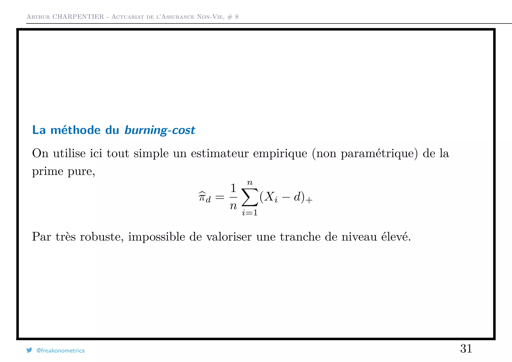
La tarification en réassurance
Le principe de base est le calcul de la prime pure, correspondant à l’espérance
mathématique des paiements, avec franchise.
Pour un traité stop-loss, de portée infinie, le montant de l’indemnité versée par le
réassureur est (X − d)+, et la prime pure est donc
E[(X − d)+] = E[(X − d)+|X ≤ d] · P[X ≤ d] + E[(X − d)+|X > d] · P[X > d],
ce qui se simplifie simplement en
πd = E[(X − d)+] = E[X − d|X > d] · P[X > d].
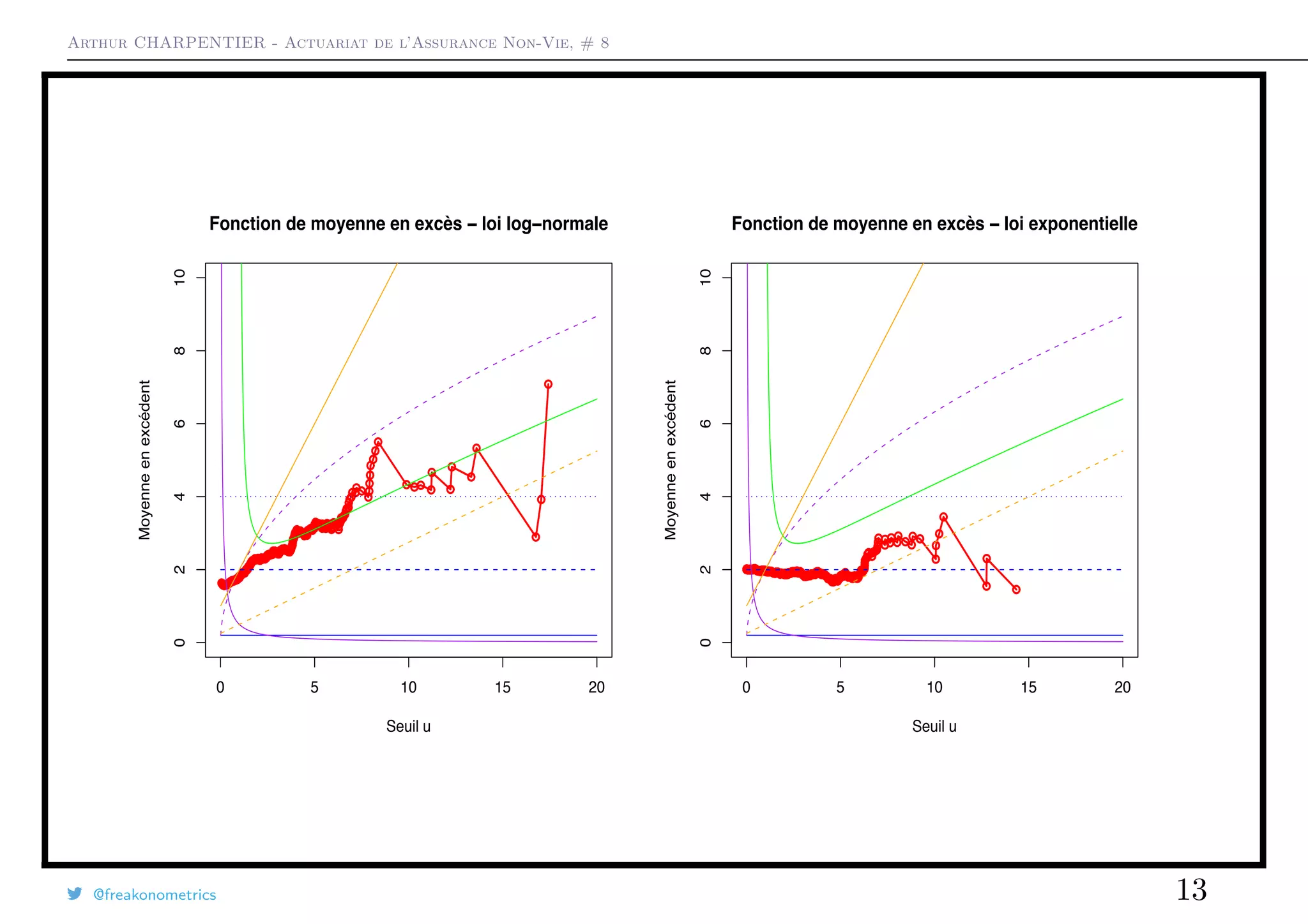
La quantité E[X − d|X > d] correspond à la fonction de moyenne en excès, notée
e(d),
e(x) =
1
P[X > x]
∞
x
P[X > t]dt.
@freakonometrics 30](https://image.slidesharecdn.com/slides-ensae-2016-8-161119144952/75/Slides-ensae-2016-8-30-2048.jpg)


![Arthur CHARPENTIER - Actuariat de l’Assurance Non-Vie, # 8
La tarification par exposition
Il s’agit ici de calculer la prime pour des traités non-proportionels.
Soit M la somme assurée. On notera xi = Xi/M les montants de sinistres (i.i.d.)
et d = D/M où D désigne la priorité du traité en excédent de sinistre. La prime
pure, du point de vue de l’assureur est
E [min {X, D}] E [N] = ME [min {x, d}] E [N]
et la prime pure dite de base sera
E [X] E [N] = ME [min {x, 1}] E [N] .
La courbe d’exposition G est le rapport entre la prime de l’assureur et la prime
de base, G : [0, 1] → [0, 1]
G (d) =
E [min {x, d}]
E [min {x, 1}]
pour d ∈ [0, 1] .
@freakonometrics 35](https://image.slidesharecdn.com/slides-ensae-2016-8-161119144952/75/Slides-ensae-2016-8-35-2048.jpg)
![Arthur CHARPENTIER - Actuariat de l’Assurance Non-Vie, # 8
La courbe d’exposition
La courbe d’exposition est définie simplement par
G(d) =
E[min{X, d}]
E([X]
=
1
E([X]
d
0
(1 − F(t))dt.
On notera que cette fonction G vérifie G(0) = 0, G(1) = 1, qu’elle est croissante
et concave. En effet,
∂G(d)
∂d
=
1 − F(d)
f(d)
≥ 0,
et
∂2
G(d)
∂d2
=
−f(d)
f(d)
≤ 0,
La concavité reflète la part des grands risques: plus la courbe est proche de la
diagonale, plus la part des grands risques dans la charge totale tend à être
négligeable.
@freakonometrics 36](https://image.slidesharecdn.com/slides-ensae-2016-8-161119144952/75/Slides-ensae-2016-8-36-2048.jpg)


![Arthur CHARPENTIER - Actuariat de l’Assurance Non-Vie, # 8
Réassurance, Exemple des Ouragans
et on obtient alors des chiffres
1 > base=db[ ,1:4]
2 > base$Base.Economic.Damage=Vectorize( stupidcomma )(db$Base.Economic.
Damage)
3 > base$Normalized.PL05=Vectorize( stupidcomma )(db$Normalized.PL05)
4 > base$Normalized.CL05=Vectorize( stupidcomma )(db$Normalized.CL05)
et on obtient la base suivante
1 > tail(base)
2 Year Hurricane. Description State Category Base.Economic.Damage
3 202 2005 Cindy LA 1 3.20e+08
4 203 2005 Dennis FL 3 2.23e+09
5 204 2005 Katrina LA ,MS 3 8.10e+10
6 205 2005 Ophelia NC 1 1.60e+09
7 206 2005 Rita TX 3 1.00e+10
8 207 2005 Wilma FL 3 2.06e+10
@freakonometrics 40](https://image.slidesharecdn.com/slides-ensae-2016-8-161119144952/75/Slides-ensae-2016-8-40-2048.jpg)
![Arthur CHARPENTIER - Actuariat de l’Assurance Non-Vie, # 8
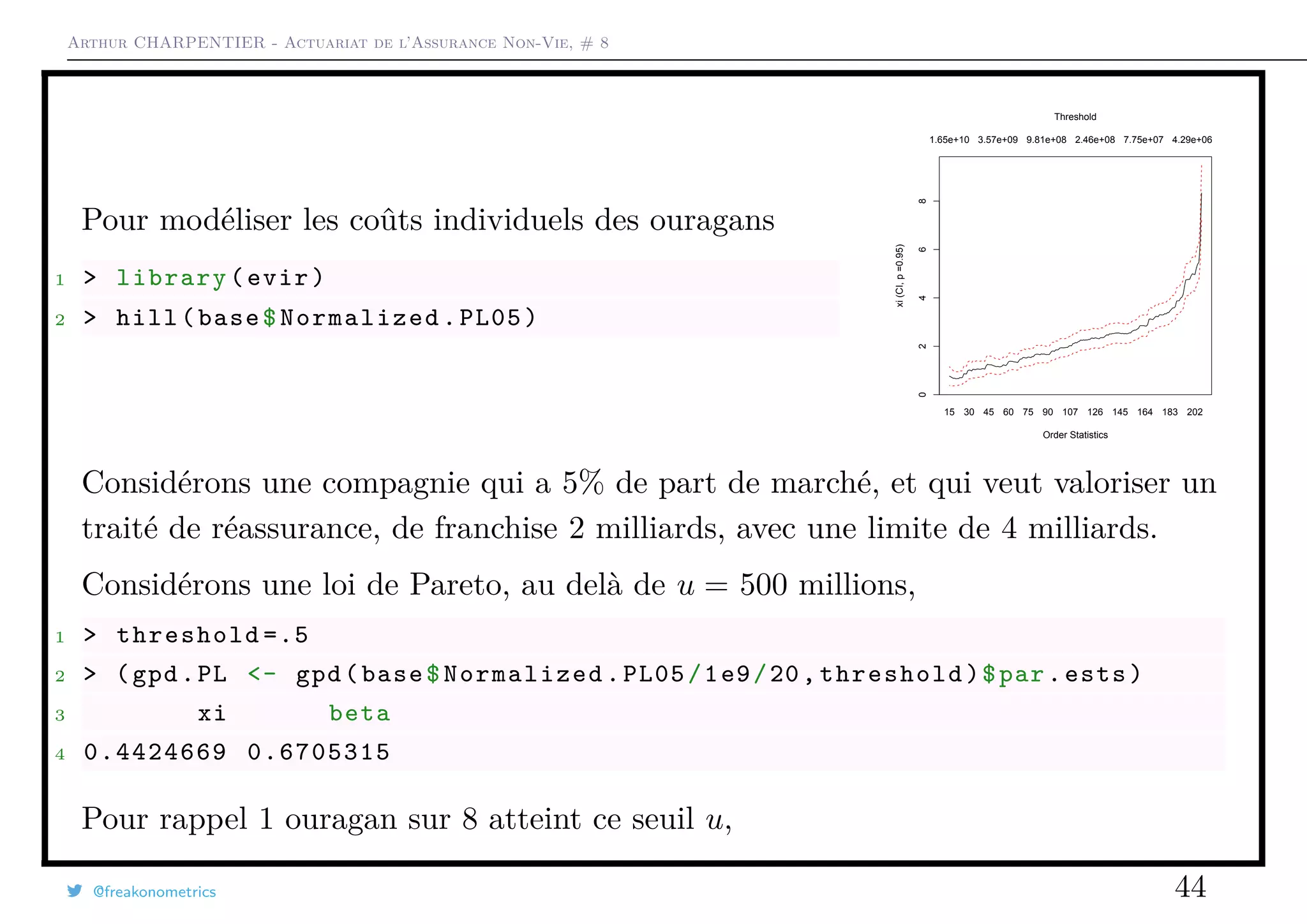
Réassurance, Exemple des Ouragans
La base historique de coûts d’ouragans est
1 > plot(base$Normalized .PL05/1e9 ,type="h",ylim=
c(0 ,155))
0 50 100 150 200
050100150
Index
L’analyse se fait (comme en assurance non-vie classique) en deux temps : on va
modéliser la fréquence annuelle, et les coûts individuels. La base des fréquence
s’obtient avec
1 > TB <- table(base$Year)
2 > years <- as.numeric(names(TB))
3 > counts <- as.numeric(TB)
4 > years0 =(1900:2005) [which(! (1900:2005)%in%years)]
5 > db <- data.frame(years=c(years ,years0),
@freakonometrics 41](https://image.slidesharecdn.com/slides-ensae-2016-8-161119144952/75/Slides-ensae-2016-8-41-2048.jpg)
![Arthur CHARPENTIER - Actuariat de l’Assurance Non-Vie, # 8
6 + counts=c(counts ,rep(0, length(years0))))
7 > db [88:93 ,]
8 years counts
9 88 2003 3
10 89 2004 6
11 90 2005 6
12 91 1902 0
13 92 1905 0
14 93 1907 0
On a, en moyenne, deux ouragans par an,
1 > mean(db$counts)begin{lstlisting }[ escapechar=
,style=mystyle,firstnumber=1][1]
1.95283
On peut aussi tenter un modèle de régression, linéaire
1 > reg0 <- glm(counts~years ,data=db ,family=poisson(link="identity"),
2 + start=lm(counts~years ,data=db)$ coefficients )
@freakonometrics 42](https://image.slidesharecdn.com/slides-ensae-2016-8-161119144952/75/Slides-ensae-2016-8-42-2048.jpg)
![Arthur CHARPENTIER - Actuariat de l’Assurance Non-Vie, # 8
ou exponentiel
1 > reg1 <- glm(counts~years ,data=db ,family=poisson(link="log"))
1 > (predictions=cbind(constant=mean(db$counts),linear= cpred0 [126] ,
exponential=cpred1 [126]))
2 constant linear exponential
3 126 1.95283 3.573999 4.379822
@freakonometrics 43](https://image.slidesharecdn.com/slides-ensae-2016-8-161119144952/75/Slides-ensae-2016-8-43-2048.jpg)
![Arthur CHARPENTIER - Actuariat de l’Assurance Non-Vie, # 8
1 > mean(base$Normalized .CL05/1e9/20 >.5)
2 [1] 0.1256039
On peu alors valoriser un contrat de réassurance To compute it we can use
1 > E <- function(yinf ,ysup ,xi ,beta){
2 + as.numeric(integrate(function(x) (x-yinf)*dgpd(x,xi ,mu=threshold ,
beta), lower=yinf ,upper=ysup)$value +(1- pgpd(ysup ,xi ,mu=threshold ,
beta))*(ysup -yinf)) }
Si on espère être touché par 2 ouragans, une année donnée
1 > predictions [1]
2 [1] 1.95283
que chaque ouragan a 12.5% de chancess de coûter plus de 500 million
1 > mean(base$Normalized .PL05/1e9/20 >.5)
2 [1] 0.1256039
et que si un ouragan dépasse 500 million, le coût moyen en excès (en millions) est
@freakonometrics 45](https://image.slidesharecdn.com/slides-ensae-2016-8-161119144952/75/Slides-ensae-2016-8-45-2048.jpg)
![Arthur CHARPENTIER - Actuariat de l’Assurance Non-Vie, # 8
1 > E(2,6,gpd.PL[1],gpd.PL [2])*1e3
2 [1] 330.9865
de telle sorte que la prime pure d’un contrat de réassurance serait
1 > predictions [1]*mean(base$Normalized.PL05/1e9/20 >.5)*
2 + E(2,6,gpd.PL[1], gpd.PL [2])*1e3
3 [1] 81.18538
en millions d’euros, pour une couverture de 4 milliards, en excès de 2.
@freakonometrics 46](https://image.slidesharecdn.com/slides-ensae-2016-8-161119144952/75/Slides-ensae-2016-8-46-2048.jpg)

![Arthur CHARPENTIER - Actuariat de l’Assurance Non-Vie, # 8
Fréquence des sinistres en Perte d’Exploitation
1 > date=db$DSUR
2 > D=as.Date(as.character(date),format="%Y%m%d"
)
3 > vD=seq(min(D),max(D),by=1)
4 > sD=table(D)
5 > d1=as.Date(names(sD))
6 > d2=vD[-which(vD%in%d1)]
7 > vecteur.date=c(d1 ,d2)
8 > vecteur.cpte=c(as.numeric(sD),rep(0, length(
d2)))
9 > base=data.frame(date=vecteur.date ,cpte=
vecteur.cpte)
1985 1990 1995 2000
05101520
Utilisons une régression de Poisson pour modéliser la fréquence journalière de
sinistres.
1 > regdate=glm(cpte~date ,data=base ,family=poisson(link="log"))
@freakonometrics 48](https://image.slidesharecdn.com/slides-ensae-2016-8-161119144952/75/Slides-ensae-2016-8-48-2048.jpg)
![Arthur CHARPENTIER - Actuariat de l’Assurance Non-Vie, # 8
2 > nd2016=data.frame(date=seq(as.Date(as.character (20160101) ,format="
%Y%m%d"),
3 + as.Date(as.character (20161231) ,format="%Y%m
%d"),by=1))
4 > pred2016 =predict(regdate ,newdata=nd2016 ,type="response")
5 > sum(pred2016)
6 [1] 163.4696
Il y a environ 165 sinistres, par an.
@freakonometrics 49](https://image.slidesharecdn.com/slides-ensae-2016-8-161119144952/75/Slides-ensae-2016-8-49-2048.jpg)

![Arthur CHARPENTIER - Actuariat de l’Assurance Non-Vie, # 8
Réassurance, Exemple de la Perte d’Exploitation
Considérons un contrat ave une franchise de 15 millions, pour une converture
totale de 35 millions. Pour la compagnie de réassurance, le coût espéré est
E(g(X)) avec
g(x) = min{35, max{x − 15, 0}}
La fonction d’indemnité est
1 > indemn=function(x) pmin ((x -15)*(x >15) ,50-15)
Sur 16 ans, l’indemnité moyenne aura été de
1 > mean(indemn(db$COUTSIN/1e6))
2 [1] 0.1624292
@freakonometrics 51](https://image.slidesharecdn.com/slides-ensae-2016-8-161119144952/75/Slides-ensae-2016-8-51-2048.jpg)
![Arthur CHARPENTIER - Actuariat de l’Assurance Non-Vie, # 8
Réassurance, Exemple de la Perte d’Exploitation
Par sinistre, la compagnie de réassurance pait, en moyenne, 162,430 euros. Donc
avec 160 sinistres par an, la prime pure - burning cost - est de l’ordre de 26
millions.
1 > mean(indemn(db$COUTSIN/1e6))*160
2 [1] 25.98867
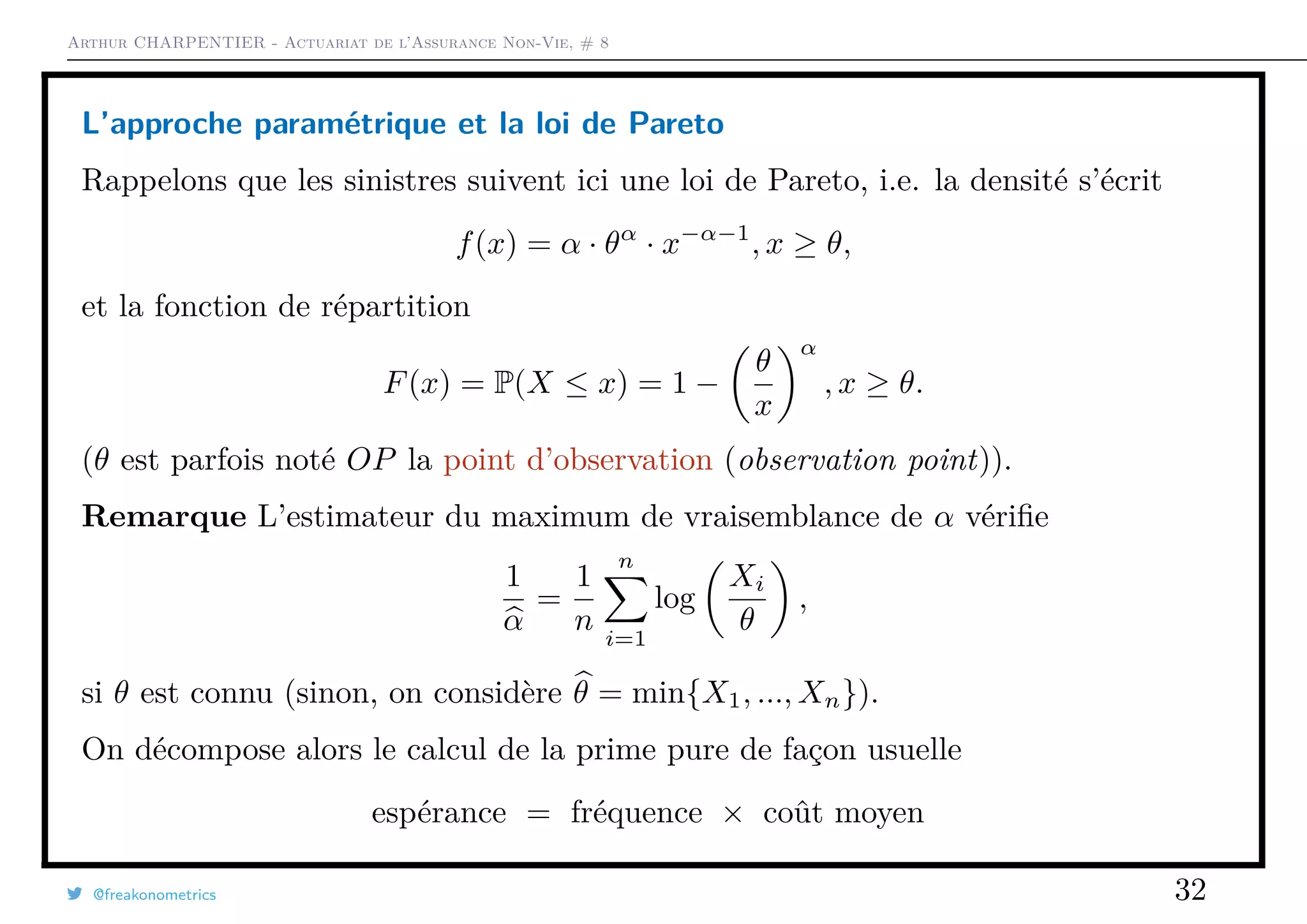
On peut aussi tenter un modèle paramétrique, de type Pareto. Les trois
paramètres sont
• le seuil µ (considéré comme fixe)
• le paramètre d’échelle (scale) σ (noté aussi β)
• the tail index ξ
@freakonometrics 52](https://image.slidesharecdn.com/slides-ensae-2016-8-161119144952/75/Slides-ensae-2016-8-52-2048.jpg)

![Arthur CHARPENTIER - Actuariat de l’Assurance Non-Vie, # 8
Réassurance, Exemple de la Perte d’Exploitation
Sachant qu’un sinistre dépasse 12 million, le remboursement moyen est de l’ordre
de 6 millions
1 > E(15e6 ,50e6 ,gpd.PL[1], gpd.PL [2] ,12e6)
2 [1] 6058125
La probabilité qu’un sinistre dépasse u est
1 > mean(db$COUTSIN >12 e6)
2 [1] 0.02639296
Aussi, avec 160 sinistres par an,
1 > p
2 [1] 159.4757
et 2.6% des sinistres qui dépassent 12 millions,
1 > mean(db$COUTSIN >12 e6)
2 [1] 0.02639296
@freakonometrics 54](https://image.slidesharecdn.com/slides-ensae-2016-8-161119144952/75/Slides-ensae-2016-8-54-2048.jpg)
![Arthur CHARPENTIER - Actuariat de l’Assurance Non-Vie, # 8
Réassurance, Exemple de la Perte d’Exploitation
Finallement, la prime pure est
1 > p*mean(db$COUTSIN >12 e6)*E(15e6 ,50e6 ,gpd.PL[1], gpd.PL[2] ,12 e6)
2 [1] 25498867
qui est proche de la valeur empirique.
On peut regarder la robustesse au choix de u,
1 > esp=function(threshold =12e6 ,p=sum(pred2010)){
2 + (gpd.PL <- gpd(db$COUTSIN ,threshold)$par.
ests)
3 + return(p*mean(db$COUTSIN >threshold)*E(15e6
,50e6 ,gpd.PL[1], gpd.PL[2], threshold))}
q
q
q
q
q
q
q q
q
q
q
q
q
q
q
2 4 6 8 10 12 14
2628303234
Threshold
Prixdelacouverture('000000)
@freakonometrics 55](https://image.slidesharecdn.com/slides-ensae-2016-8-161119144952/75/Slides-ensae-2016-8-55-2048.jpg)
![Arthur CHARPENTIER - Actuariat de l’Assurance Non-Vie, # 8
Retour aux données RC
On peut utiliser un modèle avec comme loi pour les coûts une loi de Pareto
1 > ?gamlss.family
2 > ?PARETO2
La loi de Pareto a ici pour densité
f(y|µ, σ) =
1
σ
µ
1
σ [y + µ]− 1
σ −1
et sa moyenne est alors
E[Y ] =
µσ
1 − σ
avec ici
E[Y |X = x] =
exT
α
exT
β
1 − exTβ
@freakonometrics 56](https://image.slidesharecdn.com/slides-ensae-2016-8-161119144952/75/Slides-ensae-2016-8-56-2048.jpg)
![Arthur CHARPENTIER - Actuariat de l’Assurance Non-Vie, # 8
Retour aux données RC
1 > seuil =1500
2 > regpareto=gamlss(cout~ageconducteur , sigma.formula= ~ageconducteur
,data=base_RC[base_RC$cout >seuil ,], family=PARETO2(mu.link = "log",
sigma.link = "log"))
3 -------------------------------------------------------------------
4 Mu link function: log
5 Mu Coefficients :
6 Estimate Std. Error t value Pr(>|t|)
7 (Intercept) 9.166591 0.212249 43.188 <2e-16 ***
8 ageconducteur 0.007024 0.004420 1.589 0.113
9
10 -------------------------------------------------------------------
11 Sigma link function: log
12 Sigma Coefficients :
13 Estimate Std. Error t value Pr(>|t|)
14 (Intercept) -0.793548 0.166166 -4.776 2.58e -06 ***
15 ageconducteur -0.009316 0.003513 -2.652 0.00835 **
@freakonometrics 57](https://image.slidesharecdn.com/slides-ensae-2016-8-161119144952/75/Slides-ensae-2016-8-57-2048.jpg)

This document discusses modeling and estimating extreme risks and quantiles in non-life insurance. It introduces the generalized extreme value distribution and Pickands–Balkema–de Haan theorem, which state that maximums of iid random variables converge to one of three extreme value distributions. It also discusses estimators for the shape parameter of these distributions, such as the Hill estimator, and using the generalized Pareto distribution above a threshold to estimate value-at-risk quantiles. Examples are given applying these methods to Danish fire insurance loss data.


