1) The document describes a lab experiment using MATLAB and Simulink to model differential equations and a mechanical spring-mass damper system. 2) Two differential equations and one spring-mass system were modeled to analyze the transient and steady-state response. 3) The results showed that the solutions from MATLAB and Simulink matched the expected behaviors and verified the initial and final values as well as time constants of the systems.

1. 8/31/2015 EE 481 Lab #1
Section 001
Chad Ryan Weiss & Mireille Mballa
THE PENNSYLVANIA STATE UNIVERSITY

2. 1 | P a g e
Table of Contents
Table of figures...................................................................................................................................1
Introduction.......................................................................................................................................2
OBJECTIVES ....................................................................................................................................2
METHODS.......................................................................................................................................2
Mechanical Spring Mass Damper System......................................................................................3
First Differential Equation............................................................................................................5
Second Differential Equation........................................................................................................7
Results...............................................................................................................................................9
Conclusion .......................................................................................................................................10
References.......................................................................................................................................11
Table of figures
Figure 1 Mechanical system to be analyzed..........................................................................................2
Figure 2 Simulink graphfor the mechanical system...............................................................................3
Figure 3 MATLAB graph for the mechanical system...............................................................................4
Figure 4 Simulink graphfor the first differential equation .....................................................................5
Figure 5 MATLAB graph for the first differential equation .....................................................................6
Figure 6 Simulink for the second differential equation..........................................................................7
Figure 7 MATLAB graph for the second differential equation.................................................................8

3. 2 | P a g e
Figure 1 Mechanicalsystemto be analyzed
Introduction
OBJECTIVES
In this lab we will be using MATLAB and Simulink to model a pair of differential equations as
well as one mechanical spring-mass damper system.
METHODS
For the followingdifferential equationsandspring-massdampersystem, performthe following:
A. Write the frequency domain(Laplace)equationsthatmodel the system.
B. Findthe transferfunctionthatrelatesthe displacementvariableX(s) tothe inputvariable F(s).
C. Calculate the time domainexpressionx(t)byhand,usinginverseLaplace transformtechniques.
D. Write a simple scriptinMATLAB that will generate asolutionforandplotx(t).
E. Create a simple blockdiagraminSimulinkthatcontainsasource,transferfunctionandsink;run
a Simulinksolutiontoplotx(t).
F. Verifythe plotsobtainedinMATLABand Simulinkforx(t) asfollows:
1. Doesx(t) meetthe initial conditions?
2. Doesx(t) converge tothe correct final value?
3. Doesx(t) settle afterapproximately4time constants,usingthe slowestexponential
termin the system?
4. Doesx(t) exhibitthe expectedtransientresponse (overdamped,underdamped,or
criticallydamped) foritssecondordercomponents?
MECHANICAL SYSTEM
𝑘 = 50 N/m
𝑚 = 2 kg
𝑏 = 12 N-s/m
g = 9.8 m/s2
𝑥(0) = 0 m
𝑥̇(0) = 0 m/s
DIFFERENTIAL EQUATIONS
a) 𝒙⃛( 𝒕) + 𝟏𝟔𝒙̈ ( 𝒕) + 𝟔𝟓𝒙̇ ( 𝒕) + 𝟓𝟎𝒙( 𝒕) = 𝟓𝒖( 𝒕); 𝒙( 𝟎) = 𝒙̇ ( 𝟎) = 𝒙̈ ( 𝟎) = 𝟎
b) 𝒙̈ ( 𝒕) + 𝟒𝒙̇ ( 𝒕) + 𝟒𝒙( 𝒕) = 𝒖̇ ( 𝒕) + 𝟑𝒖( 𝒕); 𝒙( 𝟎) = 𝒙̇ ( 𝟎) = 𝟎

4. 3 | P a g e
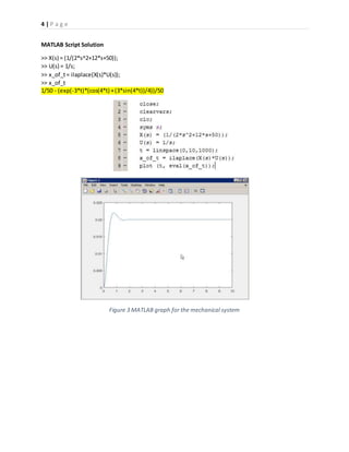
Figure 2 Simulink graph forthemechanicalsystem
Mechanical Spring Mass Damper System
𝒎𝒙̈ ( 𝒕) + 𝒃𝒙̇ ( 𝒕) + 𝒌𝒙( 𝒕) = 𝑭( 𝒕)
𝒙( 𝟎) = 𝒙̇ ( 𝟎) = 𝟎
2𝑥̈( 𝑡) + 12𝑥̇( 𝑡) + 50𝑥( 𝑡) = 𝐹( 𝑡)
2[s2
X(s)-sx(0)-x’(0)]+12[sX(s)-x(0)]+50X(s)=F(s)
[2s2
+12s+50]X(s)=F(s)
𝑋(𝑠)
𝐹(𝑠)
=
1
2𝑠2 + 12s + 50
assume F(s) = unitstep(1/s)
𝑿( 𝒔) = (
𝟏
𝒔
)(
𝟏
𝟐𝒔 𝟐+𝟏𝟐𝒔+𝟓𝟎
) (TransferFunction)
Partial Fraction Expansion
𝑋( 𝑠) =
𝐴
𝑠
+
𝐵𝑠 + 𝐶
2𝑠2 + 12𝑠 + 50
Thisrepresentsaunitstepsummedwitha generic oscillatory decay function.
A=0.02 B=-0.02 C=-0.12 a=3 ωd=4
𝑋( 𝑠) =
0.02
𝑠
−
0.02𝑠+0.12
2( 𝑠+3)2+16
𝑥( 𝑡) = [0.02 + 𝑒−3𝑡(−0.02 ∗ 𝑐𝑜𝑠(4𝑡) − 0.015 ∗ 𝑠𝑖𝑛(4𝑡))] ∗ 𝑢(𝑡)
SimulinkSolution

5. 4 | P a g e
MATLAB Script Solution
>> X(s) = (1/(2*s^2+12*s+50));
>> U(s) = 1/s;
>> x_of_t= ilaplace(X(s)*U(s));
>> x_of_t
1/50 - (exp(-3*t)*(cos(4*t) +(3*sin(4*t))/4))/50
Figure 3 MATLAB graph for the mechanical system

6. 5 | P a g e
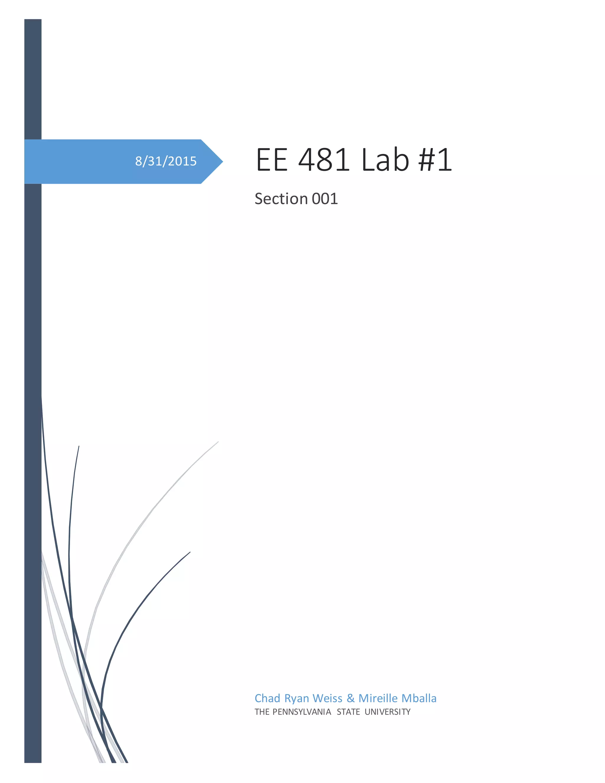
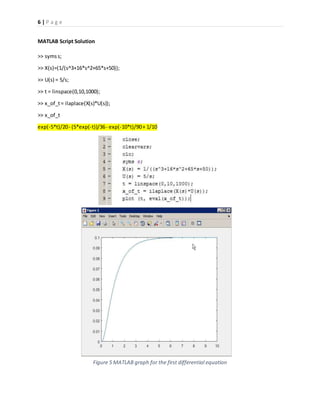
First Differential Equation
𝒙⃛( 𝒕) + 𝟏𝟔𝒙̈ ( 𝒕) + 𝟔𝟓𝒙̇ ( 𝒕) + 𝟓𝟎𝒙( 𝒕) = 𝟓𝒖( 𝒕);
𝒙( 𝟎) = 𝒙̇ ( 𝟎) = 𝒙̈ ( 𝟎) = 𝟎
[s3
X(s)+16s2
X(s)+65sX(s)+50X(s)]=5/s
Transfer Function
𝑋(𝑠)/𝑈(𝑠) = (
1
𝑠3 +16𝑠2+65𝑠+50
)
𝑋( 𝑠) = (
5
𝑠
)(
1
𝑠3 + 16𝑠2 + 65𝑠 + 50
)
Partial Fraction Expansion
𝑋( 𝑠) =
0.1
𝑠
+
−0.13
𝑠 + 1
+
0.05
𝑠 + 5
+
−0.01
𝑠 + 10
𝑥( 𝑡) = 0.1 − 0.13𝑒−𝑡 + 0.05𝑒−5𝑡 − 0.01𝑒−10𝑡
SimulinkSolution
Figure 4 Simulink graph for the first differential equation

7. 6 | P a g e
MATLAB Script Solution
>> symss;
>> X(s)=(1/(s^3+16*s^2+65*s+50));
>> U(s) = 5/s;
>> t = linspace(0,10,1000);
>> x_of_t= ilaplace(X(s)*U(s));
>> x_of_t
exp(-5*t)/20- (5*exp(-t))/36- exp(-10*t)/90+ 1/10
Figure 5 MATLAB graph for the first differential equation

8. 7 | P a g e
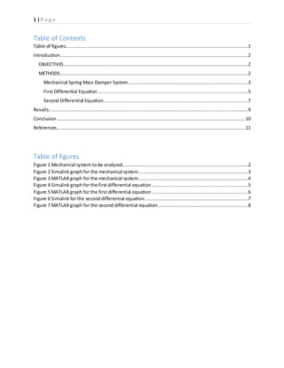
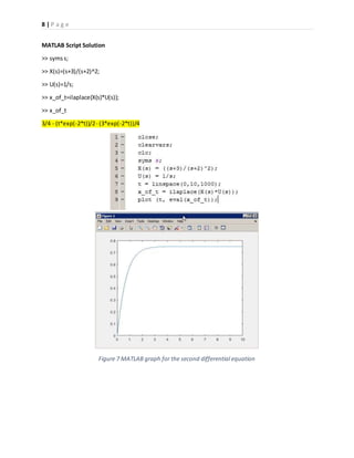
Second Differential Equation
𝒙̈ ( 𝒕) + 𝟒𝒙̇ ( 𝒕) + 𝟒𝒙( 𝒕) = 𝒖̇ ( 𝒕) + 𝟑𝒖( 𝒕)
𝒙( 𝟎) = 𝒙̇ ( 𝟎) = 𝟎
s2
X(s) + 4sX(s) + 4X(s) = sU(s) + 3U(s) [F.Domain]
(s2
+4s+4)X(s) = (s+3)U(s)
TransferFunction
𝑋(𝑠)
𝑈(𝑠)
=
(𝑠 + 3)
(𝑠2 + 4𝑠 + 4)
Partial Fraction Expansion
𝑋( 𝑠) =
0.75
𝑠
−
0.75
𝑠 + 2
−
0.5
(𝑠 + 2)^2
𝑥( 𝑡) = 0.75 − 0.75𝑒−2𝑡 − 0.5𝑡𝑒−2𝑡
SimulinkSolution
Figure 6 Simulink for the second differential equation

9. 8 | P a g e
MATLAB Script Solution
>> symss;
>> X(s)=(s+3)/(s+2)^2;
>> U(s)=1/s;
>> x_of_t=ilaplace(X(s)*U(s));
>> x_of_t
3/4 - (t*exp(-2*t))/2- (3*exp(-2*t))/4
Figure 7 MATLAB graph for the second differential equation

10. 9 | P a g e
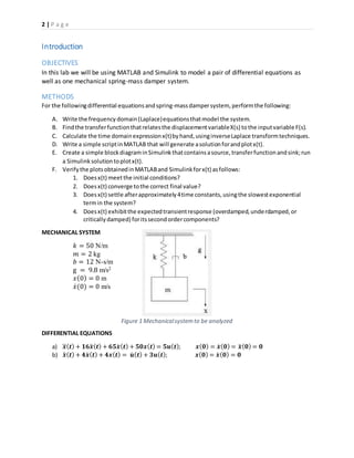
Figure 8 Simulink graph forthemechanicalsystem
≈4τ
Final value
Initial value
≈ 4τ = 2s
≈ 4τ = 4s
Initial value Initial value
Final value
Final value
Results
For our mechanical spring-massdampersystem,we obtainedthe positionof the massasa functionof
time foreveryunitintime,i.e. 𝑥( 𝑡) = [0.02 + 𝑒−3𝑡(−0.02 ∗ 𝑐𝑜𝑠(4𝑡) − 0.015 ∗ 𝑠𝑖𝑛(4𝑡))] ∗ 𝑢(𝑡).This
functioncanbe evaluatedatzeroandinfinitytodetermine ourinitialandfinal values.Bysettingt= 0,
x(0) = 0; by settingt= ∞, x(∞) =0.02 andif we take anotherlookat figure 2,we can see thatour initial
and final valuesare consistentwithoursimulation.Anotherwaytoverifyourdatais basedonthe
transientresponse orthe time constantof thisparticularsystem.The time constantforthisfunctionis
ascertainedviathe lowestdecayingexponential inthe system, (i.e.e-3t
).Time constant(τ) happenstobe
1/3 secondsforthisparticularsystem,meaningthatafterabout4τ or 1.333 seconds,the systemshould
be approximately98percentof the way to approachingthe steady-statevalue. Figure 2will verifythis.
Lastly,we knowthat the systemis underdamped due tothe complex rootsandthe simulationshowsus
justthat.
For our setof differential equations,the followingsolutionswere obtained
𝑥( 𝑡) = [0.1 − 0.13𝑒−𝑡 + 0.05𝑒−5𝑡 − 0.01𝑒−10𝑡] 𝑢 (𝑡) & 𝑥( 𝑡) = [0.75 − 0.75𝑒−2𝑡 − 0.5𝑡𝑒−2𝑡] 𝑢(𝑡).
For the two differential equation
solutionsetsshownbelow,youcan
see that the exactsame methodfor
verifyingthe datainourmechanical
spring-massdampersystemverifies
the solutionstoourdifferential
equations.Also,if we gobackand
take a look at the roots,we will see
that theyare appropriatelymatched
to theircorrespondingoutputcurves.
The leftD.E. isoverdampedandthe
rightD.E. is criticallydamped.

11. 10 | P a g e
Conclusion
In conclusion,thislabservedas anecessary introductiontomodelingsimpleandcomplex systems
(mechanical,electrical orboth). The lessonbehindthislabwasthatthere are basicallytwotypesof
systemconfigurations:open-loopandclosed-loop(feedback) systemsnotcountingcomputercontrolled
systemswhichcanapplyto eithercase (openorclosed).We alsolearnedaboutthe mainanalysisand
designobjectiveswhenitcomestocontrol systems, “analysisbeingthe processbywhichasystem’s
performance isdetermined.”[1]
Withour simulations,we wereable todetermine how the systemwouldbehave givenacertaininput.
Doingso, we were able toevaluate the transientaswell asthe steady-state response of the system.
Although there wasnodesigncomponenttothislab,we have learnedthatstabilityisthe mainobjective
and that “designisthe processbywhicha system’sperformance iscreatedorchanged”, i.e. tomaintain
or achieve stability.[1]
The resultsof thislab were thatof verysimple systems(one mechanical spring-massdampersystemand
twodifferential equations). Usingpartof the designprocess,we were able tolookata simple system
and determine the mathematical model byintegratingthe physical attributesof the systemintoan
input-outputfunctionof time calleda linear, time-invariantdifferentialequation.Withthisequationin
hand,our analysiscommenced.
Finally, we modeledandanalyzedoursystems.Knowingthatcontrol systemsare designedprimarilyfor
the purpose of stabilization,we came tothe conclusionthatnodesigneffortsneedtake place because
all of oursystem’snatural responseseventuallydecayedtozero (i.e.the systemsettledonasteady-
state value).
AfterhavingusedMATLAB& Simulink tomodel these simplesystems,we now know the basic
fundamentalsof constructingblockdiagramsandanalyzingsimple systems.Thisanalysisanddesign
practice that we have learnedinthislab will eventually allowustomodel,analyze andoptimize real-
world,future applications.

12. 11 | P a g e
References
[1] N.Nise,Control SystemsEngineering,6th
edition.New Jersey,Wiley,2011, pp. 33-116.
[2] S. vanTonningen,“EE481 – Laboratory1: UsingMATLAB andSimulinkforModelingand
Simulation,”Course Handout,2015.