This paper outlines a state variable model for a Learjet aircraft. The aircraft dynamics are modeled in both the lateral and longitudinal directions.

1. MAE 465
Flight Dynamics 2
Instructor
Dr. Marcello Napolitano
Homework # 6
State Variable Model Design
Submitted by:
Andrew Wilhelm
November 7, 2012

2. 2
Table of Contents
1 Introduction ................................................................................................................................4
2 Derivation of State Variable System .............................................................................................5
2.1 General State Variable Model...............................................................................................5
2.2 Longitudinal State Variable Model........................................................................................6
2.3 Lateral State Variable Model................................................................................................9
2.4 Augmentation of State Variable Model................................................................................12
2.4.1 Addition of Vertical Acceleration ................................................................................12
2.4.2 Addition of Altitude....................................................................................................13
2.4.3 Addition of Flight Path Angle......................................................................................14
2.4.4 Addition of Lateral Acceleration..................................................................................14
2.5 Overall State Variable Model..............................................................................................15
3 Numerical Solution of State Variable System..............................................................................17
3.1 Longitudinal State Variable Model......................................................................................17
3.2 Lateral State Variable Model..............................................................................................19
3.3 Overall State Variable Model..............................................................................................20
4 Simulation Results.....................................................................................................................23
4.1 Longitudinal Direction .......................................................................................................23
4.2 Lateral Direction................................................................................................................24
5 Sensitivity Analysis ...................................................................................................................28
5.1 Variations of 𝒄𝑳𝜶..............................................................................................................28
5.2 Variations of 𝒄𝒎𝜶.............................................................................................................29
5.3 Variations of 𝒄𝒍𝜷...............................................................................................................29
5.4 Variations of 𝒄𝒏𝜷..............................................................................................................30
5.5 Variations of 𝒄𝒎𝒖.............................................................................................................31
5.6 Variations of 𝒄𝒎𝒒.............................................................................................................32
5.7 Variations of 𝒄𝒍𝒑...............................................................................................................33
5.8 Variations of 𝒄𝒏𝒓..............................................................................................................33
6 Conclusions ..............................................................................................................................35
7.1 Reference..............................................................................................................................36
8.1 Appendix A – Simple Matlab Code for Longitudinal Direction.................................................37
8.2 Appendix B – Simple Matlab Code for Lateral Direction .........................................................41

3. 3
8.3 Appendix C – Simulink Block Diagram ..................................................................................45
8.4 Appendix D –Longitudinal Excel Spreadsheet.........................................................................46
8.5 Appendix E –Lateral Excel Spreadsheet..................................................................................50

4. 4
1 Introduction
During flight an aircraft may experience many conditions where more advance flight
control schemes are necessary. To begin this process a state variable model is derived for the
Learjet 24. This state variable model is made up of the dimensional derivatives from the aircraft.
This model allows for a multiple input multiple output system, rather than the single input single
output transfer function based method. Once the state variable model for the aircraft is found, it
is possible to run a sensitivity analysis on the aircraft. This will determine the aircraft
performance for changing aerodynamic coefficients. The conditions of this analysis will be a
Learjet 24 at maximum weight cruise conditions
Figure 1: Learjet 24

5. 5
2 Derivation of State Variable System
2.1 General State Variable Model
The first step in building the state variable model for the aircraft is to understand the
general state variable model. A general state variable model is made up of two separate sets of
equations. The first set is the state equations for the system. These equations are modeled as
shown below.
{
𝑥1̇ ( 𝑡) = 𝑓1 ((𝑥1( 𝑡), 𝑥2( 𝑡),⋯, 𝑥 𝑛( 𝑡)), (𝑢1( 𝑡), 𝑢2( 𝑡), ⋯, 𝑢 𝑚( 𝑡)))
𝑥2̇ ( 𝑡) = 𝑓2 ((𝑥1( 𝑡), 𝑥2( 𝑡),⋯ , 𝑥 𝑛( 𝑡)),(𝑢1( 𝑡), 𝑢2( 𝑡),⋯, 𝑢 𝑚( 𝑡)))
⋯
𝑥 𝑛̇ ( 𝑡) = 𝑓𝑛 ((𝑥1( 𝑡), 𝑥2( 𝑡),⋯, 𝑥 𝑛( 𝑡)), (𝑢1( 𝑡), 𝑢2( 𝑡), ⋯, 𝑢 𝑚( 𝑡)))}
Along with the state equations, the output equations must be modeled. They are shown
in the following system.
{
𝑦1( 𝑡) = 𝑔1 ((𝑥1( 𝑡), 𝑥2( 𝑡), ⋯, 𝑥 𝑛( 𝑡)), (𝑢1( 𝑡), 𝑢2( 𝑡),⋯, 𝑢 𝑚( 𝑡)))
𝑦2( 𝑡) = 𝑔2 ((𝑥1( 𝑡), 𝑥2( 𝑡), ⋯, 𝑥 𝑛( 𝑡)), (𝑢1( 𝑡), 𝑢2( 𝑡),⋯ , 𝑢 𝑚( 𝑡)))
⋯
𝑦𝑙( 𝑡) = 𝑓𝑙 ((𝑥1( 𝑡), 𝑥2( 𝑡),⋯ , 𝑥 𝑛( 𝑡)),(𝑢1( 𝑡), 𝑢2( 𝑡), ⋯, 𝑢 𝑚( 𝑡))) }
Where:
𝑛 = 𝑂𝑟𝑑𝑒𝑟 𝑜𝑓 𝑆𝑦𝑠𝑡𝑒𝑚
𝑚 = 𝑁𝑢𝑚𝑏𝑒𝑟 𝑜𝑓 𝐼𝑛𝑝𝑢𝑡
𝑙 = 𝑁𝑢𝑚𝑏𝑒𝑟 𝑜𝑓 𝑂𝑢𝑡𝑝𝑢𝑡𝑠
After the functional form of these equations is understood, they are put in matrix form.
This will produce two sets of matrices involving both the states of the system and the inputs.
The modeling of these matrices is described next.
{
𝑥1̇ ( 𝑡)
𝑥2̇ ( 𝑡)
⋯
𝑥 𝑛̇ ( 𝑡)
} = 𝐴 𝑛×𝑛
̿̿̿̿̿̿̿ {
𝑥1( 𝑡)
𝑥2( 𝑡)
⋯
𝑥 𝑙( 𝑡)
} + 𝐵 𝑛×𝑚
̿̿̿̿̿̿̿ {
𝑢1( 𝑡)
𝑢2( 𝑡)
⋯
𝑢 𝑙( 𝑡)
}
{
𝑦1 ( 𝑡)
𝑦2 ( 𝑡)
⋯
𝑦𝑙( 𝑡)
} = 𝐶𝑙×𝑛
̿̿̿̿̿̿ {
𝑥1( 𝑡)
𝑥2( 𝑡)
⋯
𝑥 𝑙( 𝑡)
} + 𝐷𝑙×𝑚
̿̿̿̿̿̿̿ {
𝑢1( 𝑡)
𝑢2( 𝑡)
⋯
𝑢 𝑙( 𝑡)
}

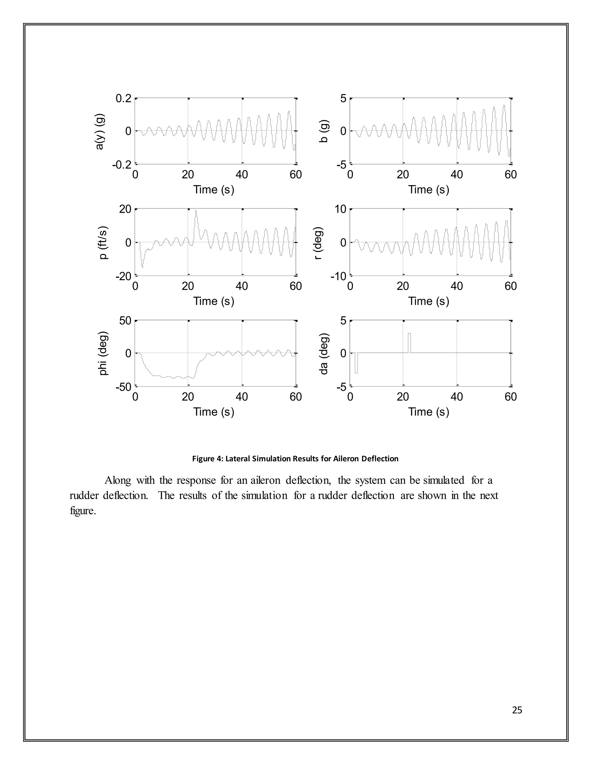
6. 6
Where:
𝐴 𝑛×𝑛
̿̿̿̿̿̿̿ = 𝑆𝑡𝑎𝑡𝑒 𝑀𝑎𝑡𝑟𝑖𝑥
𝐵 𝑛×𝑚
̿̿̿̿̿̿̿ = 𝐶𝑜𝑛𝑡𝑟𝑜𝑙 𝑀𝑎𝑡𝑟𝑖𝑥
𝐶𝑙×𝑛
̿̿̿̿̿̿ = 𝑂𝑏𝑠𝑒𝑟𝑣𝑎𝑡𝑖𝑜𝑛 𝑀𝑎𝑡𝑟𝑖𝑥
𝐷𝑙×𝑚
̿̿̿̿̿̿̿ = 𝑆𝑡𝑎𝑡𝑒 𝑀𝑎𝑡𝑟𝑖𝑥
Once the state variable matrices are understood, the system equations can be rewritten as
following.
[ 𝑥̇̅] 𝑛×1 = 𝐴 𝑛×𝑛
̿̿̿̿̿̿̿[ 𝑥̅] 𝑛×1 + 𝐵 𝑛×𝑚
̿̿̿̿̿̿̿[ 𝑢̅] 𝑚×1
[ 𝑦̅]𝑙×1 = 𝐶𝑙×𝑛
̿̿̿̿̿̿[ 𝑥̅] 𝑛×1 + 𝐷𝑙×𝑚
̿̿̿̿̿̿̿[ 𝑢̅] 𝑚×1
Now that the general state variable model is understood, it is applied to aircraft dynamics.
The model described above is applied to both the longitudinal and lateral directions of the
aircraft.
2.2 Longitudinal State Variable Model
To begin the state variable model of the longitudinal dynamics, the equations of motion
for the aircraft are necessary. These equations are made of dimensional derivatives and are
shown below.
𝑢̇ = (𝑋 𝑢 + 𝑋 𝑇𝑢
)𝑢 + 𝑋 𝛼 𝛼 − 𝑔 cos( 𝛩1) 𝜃 + 𝑋 𝛿 𝐸
𝛿 𝐸
𝑉𝑃1
𝛼̇ = 𝑍 𝑢 𝑢 + 𝑍 𝛼 𝛼 + 𝑍 𝛼̇ 𝛼̇ − 𝑔 sin( 𝛩1) 𝜃 + (𝑍 𝑞 + 𝑉𝑃1
)𝜃̇ + 𝑍 𝛿 𝐸
𝛿 𝐸
𝜃̈ = (𝑀 𝑢 + 𝑀 𝑇𝑢
)𝑢 + (𝑀 𝛼 + 𝑀 𝑇𝛼
)𝛼 + 𝑀 𝛼̇ 𝛼̇ + 𝑀 𝑞 𝜃̇ + 𝑀𝛿 𝐸
𝛿 𝐸
These sets of equations must be adjusted using the relationship shown next.
𝑞 = 𝜃̇
𝑞̇ = 𝜃̈
This yields the following system of equations.
𝑢̇ = (𝑋 𝑢 + 𝑋 𝑇𝑢
)𝑢 + 𝑋 𝛼 𝛼 − 𝑔 cos( 𝛩1) 𝜃 + 𝑋 𝛿 𝐸
𝛿 𝐸
(𝑉𝑃1
− 𝑍 𝛼̇ )𝛼̇ = 𝑍 𝑢 𝑢 + 𝑍 𝛼 𝛼 − 𝑔 sin( 𝛩1) 𝜃 + (𝑍 𝑞 + 𝑉𝑃1
)𝑞 + 𝑍 𝛿 𝐸
𝛿 𝐸
𝑞̇ = (𝑀 𝑢 + 𝑀 𝑇𝑢
)𝑢 + (𝑀 𝛼 + 𝑀 𝑇𝛼
)𝛼 + 𝑀 𝛼̇ 𝛼̇ + 𝑀 𝑞 𝑞 + 𝑀 𝛿 𝐸
𝛿 𝐸

7. 7
𝜃̇ = 𝑞
From these equations it is evident that the second equation is nested with in the third
equations of the system. Substituting and rearranging the equations yields the final system
equations for the longitudinal direction. These equations are expressed below.
𝑢̇ = (𝑋 𝑢 + 𝑋 𝑇𝑢
)𝑢 + 𝑋 𝛼 𝛼 − 𝑔 cos( 𝛩1) 𝜃 + 𝑋𝛿 𝐸
𝛿 𝐸
𝛼̇ =
𝑍 𝑢
(𝑉𝑃1
− 𝑍 𝛼̇ )
𝑢 +
𝑍 𝛼
(𝑉𝑃1
− 𝑍 𝛼̇ )
𝛼 −
𝑔 sin( 𝛩1)
(𝑉𝑃1
− 𝑍 𝛼̇ )
𝜃 +
(𝑍 𝑞 + 𝑉𝑃1
)
(𝑉𝑃1
− 𝑍 𝛼̇ )
𝑞 +
𝑍 𝛿 𝐸
(𝑉𝑃1
− 𝑍 𝛼̇ )
𝛿 𝐸
𝑞 = [𝑀 𝛼̇ (
𝑍 𝑢
(𝑉𝑃1
− 𝑍 𝛼̇ )
) + 𝑀 𝑢] 𝑢 + [𝑀 𝛼̇ (
𝑍 𝛼
(𝑉𝑃1
− 𝑍 𝛼̇ )
) + 𝑀 𝛼] 𝛼 + [𝑀 𝛼̇ (−
𝑔 sin( 𝛩1)
(𝑉𝑃1
− 𝑍 𝛼̇ )
)] 𝜃
+ [𝑀 𝛼̇ (
(𝑍 𝑞 + 𝑉𝑃1
)
(𝑉𝑃1
− 𝑍 𝛼̇ )
) + 𝑀 𝑞 ] 𝑞 + [𝑀 𝛼̇ (
𝑍 𝛿 𝐸
(𝑉𝑃1
− 𝑍 𝛼̇ )
) + 𝑀 𝛿 𝐸
] 𝛿 𝐸
𝜃̇ = 𝑞
From these equations, the primed derivatives for the aircraft are generated. They are
introduced to the above equations as shown.
𝑢̇ = 𝑋 𝑢
′
𝑢 + 𝑋 𝛼
′
𝛼 + 𝑋 𝜃
′
𝜃 + 𝑋 𝛿 𝐸
′
𝛿 𝐸
𝛼̇ = 𝑍 𝑢
′
𝑢 + 𝑍 𝛼
′
𝛼 + 𝑍 𝜃
′
𝜃 + 𝑍 𝑞
′
𝑞 + 𝑍 𝛿 𝐸
′
𝛿 𝐸
𝑞 = 𝑀 𝑢
′
𝑢 + 𝑀 𝛼
′
𝛼 + 𝑀 𝜃
′
𝜃 + 𝑀 𝑞
′
𝑞 + 𝑀 𝛿 𝐸
′
𝛿 𝐸
𝜃̇ = 𝑞
Where:
𝑋 𝑢
′
= (𝑋 𝑢 + 𝑋 𝑇𝑢
) 𝑍 𝑢
′
=
𝑍 𝑢
(𝑉𝑃1
− 𝑍 𝛼̇ )
𝑀 𝑢
′
= 𝑀 𝛼̇ (
𝑍 𝑢
(𝑉𝑃1
− 𝑍 𝛼̇ )
) + 𝑀 𝑢
𝑋 𝛼
′
= 𝑋 𝛼
𝑍 𝛼
′
=
𝑍 𝛼
(𝑉𝑃1
− 𝑍 𝛼̇ )
𝑀 𝛼
′
= 𝑀 𝛼̇ (
𝑍 𝛼
(𝑉𝑃1
− 𝑍 𝛼̇ )
) + 𝑀 𝛼
𝑋 𝜃
′
= −𝑔cos( 𝛩1) 𝑍 𝜃
′
= −
𝑔 sin( 𝛩1)
(𝑉𝑃1
− 𝑍 𝛼̇ )
𝑀 𝜃
′
= 𝑀 𝛼̇ (−
𝑔 sin( 𝛩1)
(𝑉𝑃1
− 𝑍 𝛼̇ )
)
𝑋 𝑞
′
= 0 𝑍 𝑞
′
=
(𝑍 𝑞 + 𝑉𝑃1
)
(𝑉𝑃1
− 𝑍 𝛼̇ )
𝑀 𝑞
′
= 𝑀 𝛼̇ (
(𝑍 𝑞 + 𝑉𝑃1
)
(𝑉𝑃1
− 𝑍 𝛼̇ )
) + 𝑀 𝑞
𝑋𝛿 𝐸
′
= 𝑋𝛿 𝐸
𝑍 𝛿 𝐸
′
=
𝑍 𝛿 𝐸
(𝑉𝑃1
− 𝑍 𝛼̇ )
𝑀 𝛿 𝐸
′
= 𝑀 𝛼̇ (
𝑍 𝛿 𝐸
(𝑉𝑃1
− 𝑍 𝛼̇ )
)
+ 𝑀𝛿 𝐸

8. 8
These variables represent the primed derivatives for the longitudinal dynamics. Now that
the equations of motion for the aircraft are found, the state variable model is applied. From these
equation it is evident there will be four states for the system. These states are shown in the
following formula.
𝑥 𝐿𝑜𝑛𝑔 = {
𝑢
𝛼
𝑞
𝜃
}
Along with the states, the inputs are represented by the following expression.
𝑢 𝐿𝑜𝑛𝑔 = { 𝛿 𝐸}
Once all of these expressions are understood, they are put into the state equation of the
state variable model. This is described below.
{
𝑢̇
𝛼̇
𝑞̇
𝜃̇
} = 𝐴 𝐿𝑜𝑛𝑔
̿̿̿̿̿̿̿ {
𝑢
𝛼
𝑞
𝜃
} + 𝐵 𝐿𝑜𝑛𝑔
̿̿̿̿̿̿̿{ 𝛿 𝐸}
Where:
{
𝑢̇
𝛼̇
𝑞̇
𝜃̇
} =
[
𝑋 𝑢
′
𝑋 𝛼
′
𝑋 𝑞
′
𝑋 𝜃
′
𝑍 𝑢
′
𝑍 𝛼
′
𝑍 𝑞
′
𝑍 𝜃
′
𝑀 𝑢
′
𝑀 𝛼
′
𝑀 𝑞
′
𝑀 𝜃
′
0 0 1 0 ]
{
𝑢
𝛼
𝑞
𝜃
} +
[
𝑋𝛿 𝐸
′
𝑍 𝛿 𝐸
′
𝑀 𝛿 𝐸
′
0 ]
{ 𝛿 𝐸}
The above equation is known as the state equation for the aircrafts longitudinal dynamics.
To complete the state variable model, the output equation is necessary. This is shown in the
following formula.
{
𝑢
𝛼
𝑞
𝜃
} = 𝐶 𝐿𝑜𝑛𝑔
̿̿̿̿̿̿̿ {
𝑢
𝛼
𝑞
𝜃
} + 𝐷 𝐿𝑜𝑛𝑔
̿̿̿̿̿̿̿{ 𝛿 𝐸}
Where:
{
𝑢
𝛼
𝑞
𝜃
} = [
1 0 0 0
0 1 0 0
0 0 1 0
0 0 0 1
] {
𝑢
𝛼
𝑞
𝜃
} + [
0
0
0
0
]{ 𝛿 𝐸}

9. 9
It should be noted that in this form the output of the system is equal to the state of the
system. The means the system could be controlled by a state variable feedback system. It is
possible to add an output to this equation.
2.3 Lateral State Variable Model
To begin the derivation of the lateral state variable model, the lateral directional
dynamics of the aircraft are necessary. These equations are made up of the lateral dimensional
derivatives and are expressed as follows.
(𝑉𝑃1
𝛽̇) = 𝑌𝛽 𝛽 + 𝑌𝑝 𝑝 + (𝑌𝑟 − 𝑉𝑃1
)𝑟 + 𝑔 cos( 𝛩1) 𝜙 + 𝑌𝛿 𝐴
𝛿 𝐴 + 𝑌𝛿 𝑅
𝛿 𝑅
𝑝̇ −
𝐼 𝑋𝑍
𝐼 𝑋𝑋
𝑟̇ = 𝐿 𝛽 𝛽+ 𝐿 𝑝 𝑝 + 𝐿 𝑟 𝑟 + 𝐿 𝛿 𝐴
𝛿 𝐴 + 𝐿 𝛿 𝑅
𝛿 𝑅
𝑟̇ −
𝐼 𝑋𝑍
𝐼𝑍𝑍
𝑝̇ = 𝑁𝛽 𝛽 + 𝑁 𝑝 𝑝 + 𝑁𝑟 𝑟 + 𝑁𝛿 𝐴
𝛿 𝐴 + 𝑁𝛿 𝑅
𝛿 𝑅
To simplify the moments of inertia for the aircraft, the following relationships are used.
𝐼1 =
𝐼 𝑋𝑍
𝐼 𝑋𝑋
𝐼2 =
𝐼 𝑋𝑍
𝐼𝑍𝑍
After this is done, it is evident that the second and third equations of motion are coupled.
With this in mind the second equation is rewritten. This is done in the formula below.
𝑝̇ = 𝐿 𝛽 𝛽+ 𝐿 𝑝 𝑝 + 𝐿 𝑟 𝑟 + 𝐿 𝛿 𝐴
𝛿 𝐴 + 𝐿 𝛿 𝑅
𝛿 𝑅 + 𝐼1 𝑟̇
This equation is then substituted into the third equation as shown as follows.
𝑟̇ − 𝐼2 [𝐿 𝛽 𝛽 + 𝐿 𝑝 𝑝 + 𝐿 𝑟 𝑟 + 𝐿 𝛿 𝐴
𝛿 𝐴 + 𝐿 𝛿 𝑅
𝛿 𝑅 + 𝐼1 𝑟̇] = 𝑁𝛽 𝛽 + 𝑁 𝑝 𝑝 + 𝑁𝑟 𝑟 + 𝑁 𝛿 𝐴
𝛿 𝐴 + 𝑁𝛿 𝑅
𝛿 𝑅
Solving for the state of the aircraft yields the expression below.
𝑟̇ =
(𝐼2 𝐿 𝛽 + 𝑁𝛽)
(1 − 𝐼1 𝐼2)
𝛽 +
(𝐼2 𝐿 𝑝 + 𝑁 𝑝)
(1 − 𝐼1 𝐼2)
𝑝 +
( 𝐼2 𝐿 𝑟 + 𝑁𝑟)
(1 − 𝐼1 𝐼2)
𝑟 +
(𝐼2 𝐿 𝛿 𝐴
+ 𝑁 𝛿 𝐴
)
(1 − 𝐼1 𝐼2)
𝛿 𝐴 +
(𝐼2 𝐿 𝛿 𝑅
+ 𝑁𝛿 𝑅
)
(1 − 𝐼1 𝐼2)
𝛿 𝑅
After this expression for the third equation of motion is found, it is substituted into the
second equation. This will change the second equation as follows.
𝑝̇ = (𝐿 𝛽 + 𝐼1
(𝐼2 𝐿 𝛽 + 𝑁𝛽)
(1 − 𝐼1 𝐼2)
) 𝛽 + (𝐿 𝑝 + 𝐼1
(𝐼2 𝐿 𝑝 + 𝑁 𝑝)
(1 − 𝐼1 𝐼2)
) 𝑝 + (𝐿 𝑟 + 𝐼1
( 𝐼2 𝐿 𝑟 + 𝑁𝑟)
(1 − 𝐼1 𝐼2)
) 𝑟
+ (𝐿 𝛿 𝐴
+ 𝐼1
(𝐼2 𝐿 𝛿 𝐴
+ 𝑁 𝛿 𝐴
)
(1 − 𝐼1 𝐼2)
) 𝛿 𝐴 + (𝐿 𝛿 𝑅
+ 𝐼1
(𝐼2 𝐿 𝛿 𝑅
+ 𝑁𝛿 𝑅
)
(1 − 𝐼1 𝐼2)
) 𝛿 𝑅
Which simplifies to:

10. 10
𝑝̇ =
(𝐿 𝛽 + 𝐼1 𝑁 𝛽)
(1 − 𝐼1 𝐼2)
𝛽 +
(𝐿 𝑝 + 𝐼1 𝑁 𝑝)
(1 − 𝐼1 𝐼2 )
𝑝 +
( 𝐿 𝑟 + 𝐼1 𝑁𝑟)
(1 − 𝐼1 𝐼2)
𝑟 +
(𝐿 𝛿 𝐴
+ 𝐼1 𝑁 𝛿 𝐴
)
(1 − 𝐼1 𝐼2)
𝛿 𝐴 +
(𝐿 𝛿 𝑅
+ 𝐼1 𝑁 𝛿 𝑅
)
(1 − 𝐼1 𝐼2 )
𝛿 𝑅
Once this is performed the three equations of motion for the system can be described as
shown below. Along with these equations is the following kinematic relationship for the aircraft.
𝛽̇ =
𝑌𝛽
𝑉𝑃1
𝛽 +
𝑌𝑝
𝑉𝑃1
𝑝 +
(𝑌𝑟 − 𝑉𝑃1
)
𝑉𝑃1
𝑟 +
𝑔 cos( 𝛩1)
𝑉𝑃1
𝜙 +
𝑌𝛿 𝐴
𝑉𝑃1
𝛿 𝐴 +
𝑌𝛿 𝑅
𝑉𝑃1
𝛿 𝑅
𝑝̇ =
(𝐿 𝛽 + 𝐼1 𝑁 𝛽)
(1 − 𝐼1 𝐼2)
𝛽 +
(𝐿 𝑝 + 𝐼1 𝑁 𝑝)
(1 − 𝐼1 𝐼2 )
𝑝 +
( 𝐿 𝑟 + 𝐼1 𝑁𝑟)
(1 − 𝐼1 𝐼2)
𝑟 +
(𝐿 𝛿 𝐴
+ 𝐼1 𝑁 𝛿 𝐴
)
(1 − 𝐼1 𝐼2)
𝛿 𝐴 +
(𝐿 𝛿 𝑅
+ 𝐼1 𝑁 𝛿 𝑅
)
(1 − 𝐼1 𝐼2 )
𝛿 𝑅
𝑟̇ =
(𝐼2 𝐿 𝛽 + 𝑁𝛽)
(1 − 𝐼1 𝐼2)
𝛽 +
(𝐼2 𝐿 𝑝 + 𝑁 𝑝)
(1 − 𝐼1 𝐼2)
𝑝 +
( 𝐼2 𝐿 𝑟 + 𝑁𝑟)
(1 − 𝐼1 𝐼2)
𝑟 +
(𝐼2 𝐿 𝛿 𝐴
+ 𝑁 𝛿 𝐴
)
(1 − 𝐼1 𝐼2)
𝛿 𝐴 +
(𝐼2 𝐿 𝛿 𝑅
+ 𝑁𝛿 𝑅
)
(1 − 𝐼1 𝐼2)
𝛿 𝑅
𝜙̇ = 𝑝 + tan( 𝛩1) 𝑟
These equations are the start of the state variable model. To begin this model, the single
primed derivatives must be inserted into the equations derived above. This is done as shown as
follows.
𝛽̇ = 𝑌𝛽
′
𝛽 + 𝑌𝑝
′
𝑝 + 𝑌𝑟
′
𝑟 + 𝑌𝜙
′
𝜙 + 𝑌𝛿 𝐴
′
𝛿 𝐴 + 𝑌𝛿 𝐴
′
𝛿 𝑅
𝑝̇ = 𝐿 𝛽
′
𝛽 + 𝐿 𝑝
′
𝑝+ 𝐿 𝑟
′
𝑟 + 𝐿 𝛿 𝐴
′
𝛿𝐴 + 𝐿 𝛿 𝑅
′
𝛿 𝑅
𝑟̇ = 𝑁𝛽
′
𝛽 + 𝑁 𝑝
′
𝑝 + 𝑁𝑟
′
𝑟 + 𝑁𝛿 𝐴
′
𝛿 𝐴 + 𝑁𝛿 𝑅
′
𝛿 𝑅
Where:
𝑌𝛽
′
=
𝑌𝛽
𝑉𝑃1
𝐿 𝛽
′
=
(𝐿 𝛽 + 𝐼1 𝑁 𝛽)
(1 − 𝐼1 𝐼2)
𝑁𝛽
′
=
(𝐼2 𝐿 𝛽 + 𝑁𝛽)
(1 − 𝐼1 𝐼2)
𝑌𝑝
′
=
𝑌𝑝
𝑉𝑃1
𝐿 𝑝
′
=
(𝐿 𝑝 + 𝐼1 𝑁 𝑝)
(1 − 𝐼1 𝐼2)
𝑁 𝑝
′
=
(𝐼2 𝐿 𝑝 + 𝑁 𝑝)
(1 − 𝐼1 𝐼2)
𝑌𝑟
′
=
(𝑌𝑟 − 𝑉𝑃1
)
𝑉𝑃1
𝐿 𝑟
′
=
( 𝐿 𝑟 + 𝐼1 𝑁𝑟)
(1 − 𝐼1 𝐼2 )
𝑁𝑟
′
=
( 𝐼2 𝐿 𝑟 + 𝑁𝑟)
(1 − 𝐼1 𝐼2)
𝑌𝜙
′
=
𝑔 cos( 𝛩1)
𝑉𝑃1
𝐿 𝛿 𝐴
′
=
(𝐿 𝛿 𝐴
+ 𝐼1 𝑁 𝛿 𝐴
)
(1 − 𝐼1 𝐼2)
𝑁𝛿 𝐴
′
=
(𝐼2 𝐿 𝛿 𝐴
+ 𝑁𝛿 𝐴
)
(1 − 𝐼1 𝐼2)
𝑌𝛿 𝐴
′
=
𝑌𝛿 𝐴
𝑉𝑃1
𝐿 𝛿 𝑅
′
=
(𝐿 𝛿 𝑅
+ 𝐼1 𝑁 𝛿 𝑅
)
(1 − 𝐼1 𝐼2)
𝑁 𝛿 𝑅
′
=
(𝐼2 𝐿 𝛿 𝑅
+ 𝑁𝛿 𝑅
)
(1 − 𝐼1 𝐼2)
𝑌𝛿 𝐴
′
=
𝑌𝛿 𝑅
𝑉𝑃1

11. 11
These variables represent the primed derivatives for the longitudinal dynamics. Now that
the equations of motion for the aircraft are found, the state variable model is applied. From these
equation it is evident there will be four states for the system. These states are shown in the
following formula.
𝑥 𝐿𝑎𝑡 = {
𝛽
𝑝
𝑟
𝜙
}
Along with the states, the inputs are represented by the following expression.
𝑢 𝐿𝑎𝑡 = {
𝛿 𝐴
𝛿 𝑅
}
Once all of these expressions are understood, they are put into the state equation of the
state variable model. This is described below.
{
𝛽̇
𝑝̇
𝑟̇
𝜙̇}
= 𝐴 𝐿𝑎𝑡
̿̿̿̿̿̿{
𝛽
𝑝
𝑟
𝜙
} + 𝐵 𝐿𝑎𝑡
̿̿̿̿̿̿ {
𝛿 𝐴
𝛿 𝑅
}
Where:
{
𝛽̇
𝑝̇
𝑟̇
𝜙̇}
=
[
𝑌𝛽
′
𝑌𝑝
′
𝑌𝑟
′
𝑌𝜙
′
𝐿 𝛽
′
𝐿 𝑝
′
𝐿 𝑟
′
0
𝑁𝛽
′
𝑁 𝑝
′
𝑁𝑟
′
0
0 1 tan( 𝛩1) 0 ]
{
𝛽
𝑝
𝑟
𝜙
} +
[
𝑌𝛿 𝐴
′
𝑌𝛿 𝑅
′
𝐿 𝛿 𝐴
′
𝐿 𝑅
′
𝑁 𝛿 𝐴
′
𝑁𝛿 𝑅
′
0 0 ]
{
𝛿 𝐴
𝛿 𝑅
}
The above equation is known as the state equation for the aircrafts lateral dynamics. To
complete the state variable model, the output equation is necessary. This is shown in the
following formula.
{
𝛽
𝑝
𝑟
𝜙
} = 𝐶 𝐿𝑜𝑛𝑔
̿̿̿̿̿̿̿ {
𝛽
𝑝
𝑟
𝜙
} + 𝐷 𝐿𝑜𝑛𝑔
̿̿̿̿̿̿̿{
𝛿 𝐴
𝛿 𝑅
}
Where:
{
𝛽
𝑝
𝑟
𝜙
} = [
1 0 0 0
0 1 0 0
0 0 1 0
0 0 0 1
]{
𝛽
𝑝
𝑟
𝜙
} + [
0 0
0 0
0 0
0 0
]{
𝛿 𝐴
𝛿 𝑅
}

12. 12
2.4 Augmentation of State Variable Model
2.4.1 Addition of Vertical Acceleration
Once the generic longitudinal state variable model is known, it is possible to add and
addition output for the system. This addition, although, must be a function of the state of the
system. To do this basic physics is used to derive the acceleration in the vertical direction for the
aircraft. This is represented in the following formula.
𝛼 𝑍 =
∑ 𝑓𝑍
𝑚
First the conservation of linear momentum equation in the z-direction must be found.
This equation is shown below.
(𝑓𝐴 𝑍
+ 𝑓𝑇𝑧
) = 𝑚[𝑉𝑃1
𝛼̇ − 𝑉𝑝1
𝑞] + 𝑚𝑔 sin( 𝛩1) 𝜃 − 𝑚𝑔 sin( 𝛩1)
Combining these equations yields:
𝛼 𝑍 =
∑ 𝑓𝑍
𝑚
=
𝑚[𝑉𝑃1
𝛼̇ − 𝑉𝑝1
𝑞] + 𝑚𝑔 sin( 𝛩1) 𝜃 − 𝑚𝑔 sin( 𝛩1)
𝑚
Which reduces to:
𝛼 𝑍 = [𝑉𝑃1
𝛼̇ − 𝑉𝑝1
𝑞] + 𝑔 sin( 𝛩1) 𝜃 − 𝑔 sin( 𝛩1)
After this equation is found, it should be noted that the “𝛼̇” equation derived above is
nested inside the equation. This changes the formula as shown below.
𝛼 𝑍 = [𝑉𝑃1
(𝑍 𝑢
′
𝑢 + 𝑍 𝛼
′
𝛼 + 𝑍 𝜃
′
𝜃 + 𝑍 𝑞
′
𝑞 + 𝑍 𝛿 𝐸
′
𝛿 𝐸) − 𝑉𝑝1
𝑞] + 𝑔 sin( 𝛩1) 𝜃 − 𝑔sin( 𝛩1) 𝛼
This equation reduces to the following.
𝛼 𝑍 = [𝑉𝑃1
𝑍 𝑢
′
𝑢 + 𝑉𝑃1
𝑍 𝛼
′
𝛼 − 𝑔 sin( 𝛩1) 𝛼 + 𝑉𝑃1
𝑍 𝜃
′
𝜃 + 𝑔sin( 𝛩1) 𝜃 + 𝑉𝑃1
𝑍 𝑞
′
𝑞 − 𝑉𝑝1
𝑞 + 𝑉𝑃1
𝑍𝛿 𝐸
′
𝛿 𝐸]
= (𝑉𝑃1
𝑍 𝑢
′
)𝑢 + (𝑉𝑃1
𝑍 𝛼
′
− 𝑔sin( 𝛩1))𝛼 + (𝑉𝑃1
𝑍 𝜃
′
+ 𝑔 sin( 𝛩1))𝜃 + (𝑉𝑃1
𝑍 𝑞
′
− 𝑉𝑝1
)𝑞 + (𝑉𝑃1
𝑍 𝛿 𝐸
′
)𝛿 𝐸
Once this equation is found, it is possible to add the double prime derivatives into the
expression. This is shown below.
𝛼 𝑍 = 𝑍 𝑢
′′
𝑢 + 𝑍 𝛼
′′
𝛼 + 𝑍 𝜃
′′
𝜃 + 𝑍 𝑞
′′
𝑞 + 𝑍 𝛿 𝐸
′′
𝛿 𝐸
Where:
𝑍 𝑢
′′
= 𝑉𝑃1
𝑍 𝑢
′
𝑍 𝛼
′′
= 𝑉𝑃1
𝑍 𝛼
′
− 𝑔 sin( 𝛩1)
𝑍 𝜃
′′
= 𝑉𝑃1
𝑍 𝜃
′
+ 𝑔 sin( 𝛩1) 𝑍 𝑞
′′
= 𝑉𝑃1
𝑍 𝑞
′
− 𝑉𝑝1
𝑍 𝛿 𝐸
′′
= 𝑉𝑃1
𝑍 𝛿 𝐸
′

13. 13
These derivatives are added to the output equation for the system. The changes to the
output equation are expressed as follows.
{
𝛼 𝑧
𝑢
𝛼
𝑞
𝜃 }
=
[
𝑍 𝑢
′′
𝑍 𝛼
′′
𝑍 𝑞
′′
𝑍 𝜃
′′
1 0 0 0
0 1 0 0
0 0 1 0
0 0 0 1 ]
{
𝑢
𝛼
𝑞
𝜃
} +
[
𝑍 𝛿 𝐸
′′
0
0
0
0 ]
{ 𝛿 𝐸}
2.4.2 Addition of Altitude
Adding altitude to the longitudinal dynamics requires the derivation of the flight path
equations for an aircraft. These equations are shown in the following matrix.
(
𝑋̇ ′
𝑌̇ ′
𝑍̇ ′
)
= [
cos 𝛹 cos 𝛩 − sin 𝛹 cos 𝛷 + cos 𝛹 sin 𝛩 sin 𝛷 sin 𝛹 sin 𝛷 + cos 𝛹 sin 𝛩 cos 𝛷
sin 𝛹 cos 𝛩 cos 𝛹 cos 𝛷 + sin 𝛹 sin 𝛩 sin 𝛷 −sin 𝛷 cos 𝛹 + sin 𝛹 sin 𝛩 cos 𝛷
− sin 𝛩 cos 𝛩 sin 𝛷 cos 𝛩 cos 𝛷
] (
𝑈
𝑉
𝑊
)
To add altitude to the outputs only the trajectory in the z-direction is necessary. The
expression for altitude is the negative trajectory in the z-direction. This is expressed
mathematically below.
ℎ̇ = −𝑍̇ ′
= 𝑈 sin 𝛩 − 𝑉 cos 𝛩 sin 𝛷 − 𝑊 cos 𝛩 cos 𝛷
Using the small perturbations assumption for the aircraft, the above equation is reduced
as such.
ℎ̇ = −𝑍̇ ′
= 𝑉𝑃1
θ − 𝑤
Where:
𝑤 = 𝑉𝑃1
𝛼
Yielding:
ℎ̇ = −𝑍̇′
= 𝑉𝑃1
𝜃 − 𝑉𝑃1
𝛼 = 𝑉𝑃1
( 𝜃 − 𝛼)
Once this expression is found, it is possible to add this equation to the longitudinal state
variable model for the aircraft. This is represented in the state matrix below.

14. 14
{
𝑢̇
𝛼̇
𝑞̇
𝜃̇
ℎ̇ }
=
[
𝑋 𝑢
′
𝑋 𝛼
′
𝑋 𝑞
′
𝑋 𝜃
′
0
𝑍 𝑢
′
𝑍 𝛼
′
𝑍 𝑞
′
𝑍 𝜃
′
0
𝑀 𝑢
′
𝑀 𝛼
′
𝑀 𝑞
′
𝑀 𝜃
′
0
0 0 1 0 0
0 −𝑉𝑃1
0 𝑉𝑃1
0]{
𝑢
𝛼
𝑞
𝜃
ℎ}
+
[
𝑋 𝛿 𝐸
′
𝑍 𝛿 𝐸
′
𝑀𝛿 𝐸
′
0
0 ]
{ 𝛿 𝐸}
2.4.3 Addition of Flight Path Angle
To add the flight path angle of the aircraft to the state variable model, this angle must be
modeled with respect to the state variables. This is done in the following formula.
𝛾 = 𝜃 − 𝛼
This changes the output matrix of the longitudinal state variable model as such.
{
𝑢
𝛼
𝑞
𝜃
𝛾}
=
[
1 0 0 0
0 1 0 0
0 0 1 0
0 0 0 1
0 −1 0 1]
{
𝑢
𝛼
𝑞
𝜃
} +
[
0
0
0
0
0]
{ 𝛿 𝐸}
2.4.4 Addition of Lateral Acceleration
To add the lateral velocity to the outputs of the lateral state variable model, basic physics
are followed. They derive the acceleration in the lateral direction for the aircraft. This is
represented in the following formula.
𝛼 𝑌 =
∑ 𝑓𝑌
𝑚
First the conservation of linear momentum equation in the z-direction must be found.
This equation is shown below.
(𝑓𝐴 𝑌
+ 𝑓𝑇𝑌
) = 𝑚[𝑉𝑃1
𝛽̇ − 𝑉𝑝1
𝑟] − 𝑚𝑔 cos( 𝛩1) 𝜙
Combining these equations yields:
𝛼 𝑌 =
∑ 𝑓𝑌
𝑚
=
𝑚[𝑉𝑃1
𝛽̇ − 𝑉𝑝1
𝑟] − 𝑚𝑔 cos( 𝛩1) 𝜙
𝑚
Which reduces to:
𝛼 𝑌 = [𝑉𝑃1
𝛽̇ − 𝑉𝑝1
𝑟] − 𝑔cos( 𝛩1) 𝜙
After this equation is found, it should be noted that the “𝛽̇” equation derived above is
nested inside the equation. This changes the formula as shown below.
𝛼 𝑌 = [𝑉𝑃1
(𝑌𝛽
′
𝛽 + 𝑌𝑝
′
𝑝 + 𝑌𝑟
′
𝑟 + 𝑌𝜙
′
𝜙 + 𝑌𝛿 𝐴
′
𝛿 𝐴 + 𝑌𝛿 𝐴
′
𝛿 𝑅) − 𝑉𝑝1
𝑟] − 𝑔 cos( 𝛩1) 𝜙

15. 15
This equation reduces to the following.
𝛼 𝑌 = (𝑉𝑃1
𝑌𝛽
′
)𝛽+ (𝑉𝑃1
𝑌𝑝
′
)𝑝 + (𝑉𝑃1
( 𝑌𝑟
′
+ 1)) 𝑟 + (𝑉𝑃1
(𝑌𝜙
′
− 𝑔cos( 𝛩1))) 𝜙 + (𝑉𝑃1
𝑌𝛿 𝐴
′
)𝛿 𝐴
+ (𝑉𝑃1
𝑌𝛿 𝑅
′
)𝛿 𝑅
Once this equation is found, it is possible to add the double prime derivatives into the
expression. This is shown below.
𝛼 𝑌 = 𝑌𝛽
′′
𝛽 + 𝑌𝑝
′′
𝑝+ 𝑌𝑟
′′
𝑟+ 𝑌𝜙
′′
𝜙 + 𝑌𝛿 𝐴
′′
𝛿 𝐴 + 𝑌𝛿 𝑅
′′
𝛿 𝑅
Where:
𝑌𝛽
′′
= 𝑉𝑃1
𝑌𝛽
′
𝑌𝜙
′′
= 𝑉𝑃1
(𝑌𝜙
′
− 𝑔cos( 𝛩1))
𝑌𝑝
′′
= 𝑉𝑃1
𝑌𝑝
′ 𝑌𝛿 𝐴
′′
= 𝑉𝑃1
𝑌𝛿 𝐴
′
𝑌𝑟
′′
= 𝑉𝑃1
( 𝑌𝑟
′
+ 1) 𝑌𝛿 𝑅
′′
= 𝑉𝑃1
𝑌𝛿 𝑅
′
These derivatives are added to the output equation for the system. The changes to the
output equation are expressed as follows.
{
𝛼 𝑌
𝛽
𝑝
𝑟
𝜙 }
=
[
𝑌𝛽
′′
𝑌𝑝
′′
𝑌𝑟
′′
𝑌𝜙
′′
1 0 0 0
0 1 0 0
0 0 1 0
0 0 0 1 ]
{
𝛽
𝑝
𝑟
𝜙
} +
[
𝑌𝛿 𝐴
′′
𝑌𝛿 𝑅
′′
0 0
0 0
0 0
0 0 ]
{
𝛿 𝐴
𝛿 𝑅
}
2.5 Overall State Variable Model
After the augmentation of the state variable model is understood, the overall system can
be shown in one model. This is described for the state equation as shown below.
{
𝑢̇
𝛼̇
𝑞̇
𝜃̇
𝛽̇
𝑝̇
𝑟̇
𝜙̇ }
=
{
𝑋 𝑢
′
𝑋 𝛼
′
𝑋 𝑞
′
𝑋 𝜃
′
0 0 0 0
𝑍 𝑢
′
𝑍 𝛼
′
𝑍 𝑞
′
𝑍 𝜃
′
0 0 0 0
𝑀 𝑢
′
𝑀 𝛼
′
𝑀 𝑞
′
𝑀 𝜃
′
0 0 0 0
0 0 1 0 0 0 0 0
0 0 0 0 𝑌𝛽
′
𝑌𝑝
′
𝑌𝑟
′
𝑌𝜙
′
0 0 0 0 𝐿 𝛽
′
𝐿 𝑝
′
𝐿 𝑟
′
0
0 0 0 0 𝑁𝛽
′
𝑁 𝑝
′
𝑁𝑟
′
0
0 0 0 0 0 1 tan( 𝛩1) 0 }
{
𝑢
𝛼
𝑞
𝜃
𝛽
𝑝
𝑟
𝜙}
+
{
𝑋𝛿 𝐸
′
𝑍 𝛿 𝐸
′
𝑀 𝛿 𝐸
′
0
0 0
0 0
0 0
0 0
0
0
0
0
𝑌𝛿 𝐴
′
𝑌𝛿 𝑅
′
𝐿 𝛿 𝐴
′
𝐿 𝑅
′
𝑁 𝛿 𝐴
′
𝑁𝛿 𝑅
′
0 0 }
{
𝛿 𝐸
𝛿 𝐴
𝛿 𝑅
}

16. 16
{
𝛼 𝑍
𝑢
𝛼
𝑞
𝜃
𝛼 𝑌
𝛽
𝑝
𝑟
𝜙 }
=
{
𝑍 𝑢
′′
𝑍 𝛼
′′
𝑍 𝑞
′′
𝑍 𝜃
′′
1 0 0 0
0 1 0 0
0 0 1 0
0 0 0 1
0 0 0 0
0 0 0 0
0 0 0 0
0 0 0 0
0 0 0 0
0 0 0 0
0 0 0 0
0 0 0 0
0 0 0 0
0 0 0 0
𝑌𝛽
′′
𝑌𝑝
′′
𝑌𝑟
′′
𝑌𝜙
′′
1 0 0 0
0 1 0 0
0 0 1 0
0 0 0 1 }
{
𝑢
𝛼
𝑞
𝜃
𝛽
𝑝
𝑟
𝜙}
+
{
𝑍 𝛿 𝐸
′′
0
0
0
0
0 0
0 0
0 0
0 0
0 0
0
0
0
0
0
𝑌𝛿 𝐴
′′
𝑌𝛿 𝑅
′′
0 0
0 0
0 0
0 0 }
{
𝛿 𝐸
𝛿 𝐴
𝛿 𝑅
}
These matrices can be reduced as follows.
{
𝑢̇
𝛼̇
𝑞̇
𝜃̇
𝛽̇
𝑝̇
𝑟̇
𝜙̇ }
= {
𝐴 𝐿𝑜𝑛𝑔 0
0 𝐴 𝐿𝑎𝑡
}
{
𝑢
𝛼
𝑞
𝜃
𝛽
𝑝
𝑟
𝜙}
+ {
𝐵 𝐿𝑜𝑛𝑔 0
0 𝐵 𝐿𝑎𝑡
} {
𝛿 𝐸
𝛿 𝐴
𝛿 𝑅
}
{
𝛼 𝑍
𝑢
𝛼
𝑞
𝜃
𝛼 𝑌
𝛽
𝑝
𝑟
𝜙 }
= {
𝐶 𝐿𝑜𝑛𝑔 0
0 𝐶 𝐿𝑎𝑡
}
{
𝑢
𝛼
𝑞
𝜃
𝛽
𝑝
𝑟
𝜙}
+ {
𝐷 𝐿𝑜𝑛𝑔 0
0 𝐷 𝐿𝑎𝑡
}{
𝛿 𝐸
𝛿 𝐴
𝛿 𝑅
}

17. 17
3 Numerical Solution of State Variable System
3.1 Longitudinal State Variable Model
When solving the state variable model for the longitudinal direction, a set of steps is
carried out. First, the dimensional derivatives for the aircraft must be known. These derivatives
are from the aircraft dynamics and are shown in the table below.
Table 1: Longitudinal Stability and Control Derivatives
Longitudinal Stability and Control Derivatives
𝑋 𝑢 -0.0194 𝑍 𝑢 -0.1382 𝑀 𝑢 0
𝑋 𝑇𝑢
-0.0003 𝑍 𝛼 -450.4 𝑀 𝑇𝑢
0
𝑋 𝛼 8.4349 𝑍 𝛼̇ -0.8721 𝑀 𝛼 -7.377
𝑋𝛿 𝐸
0 𝑍 𝑞 -1.863 𝑀 𝑇𝛼
0
𝑍 𝛿 𝐸
-35.27 𝑀 𝛼̇ -0.3993
𝑀 𝑞 -0.9237
𝑀 𝛿 𝐸
-14.29
After these values are found, the single primed derivatives for the state variable model
are needed. These values are defined as follows.
Table 2: Longitudinal Single Primed Derivatives
Longitudinal Single Primed Derivatives
𝑋 𝑢
′
-0.0197 𝑍 𝑢
′
0 𝑀 𝑢
′
0
𝑋 𝛼
′
8.435 𝑍 𝛼
′
-0.6644 𝑀 𝛼
′
-7.112
𝑋 𝜃
′ -32.16 𝑍 𝜃
′ -0.0022 𝑀 𝜃
′ 0
𝑋 𝑞
′
0 𝑍 𝑞
′
0.9960 𝑀 𝑞
′
-1.321
𝑋𝛿 𝐸
′
0 𝑍 𝛿 𝐸
′
-0.0520 𝑀 𝛿 𝐸
′
-14.27
The state equation for aircraft is generated from these derivatives. The state equation is
shown in the next formula.

18. 18
{
𝑢̇
𝛼̇
𝑞̇
𝜃̇
} = [
−0.0197 8.435 0 −32.16
0 −0.6644 0.9960 −0.0022
0 −7.112 −1.321 0
0 0 1 0
]{
𝑢
𝛼
𝑞
𝜃
} + [
0
−0.0520
−14.27
0
]{ 𝛿 𝐸}
Augmenting this equation to contain the altitude of the aircraft expands the matrix as
such.
{
𝑢̇
𝛼̇
𝑞̇
𝜃̇
ℎ̇ }
=
[
−0.0197 8.435 0 −32.16 0
0 −0.6644 0.9960 −0.0022 0
0 −7.112 −1.321 0 0
0 0 1 0 0
0 −677 0 677 0]{
𝑢
𝛼
𝑞
𝜃
ℎ}
+
[
0
−0.0520
−14.27
0
0 ]
{ 𝛿 𝐸}
After the state equation is found, the output equation is necessary. The basic output
equation for the aircraft is shown below.
{
𝑢
𝛼
𝑞
𝜃
} = [
1 0 0 0
0 1 0 0
0 0 1 0
0 0 0 1
] {
𝑢
𝛼
𝑞
𝜃
} + [
0
0
0
0
]{ 𝛿 𝐸}
Similar to the state equation, the equation is augmented to include more outputs. The
first addition to the output equation is the vertical acceleration. The first step in including this in
the output equation is solving for the double primed derivatives for the aircraft. These values are
shown in the following table.
Table 3: Longitudinal Double Primed Derivatives
Longitudinal Double Primed Derivatives
𝑍 𝑢
′′
-0.1380 𝑍 𝜃
′′
0.0020
𝑍 𝛼
′′
-451.3 𝑍 𝛿 𝐸
′′
-35.23
𝑍 𝑞
′′
-2.731
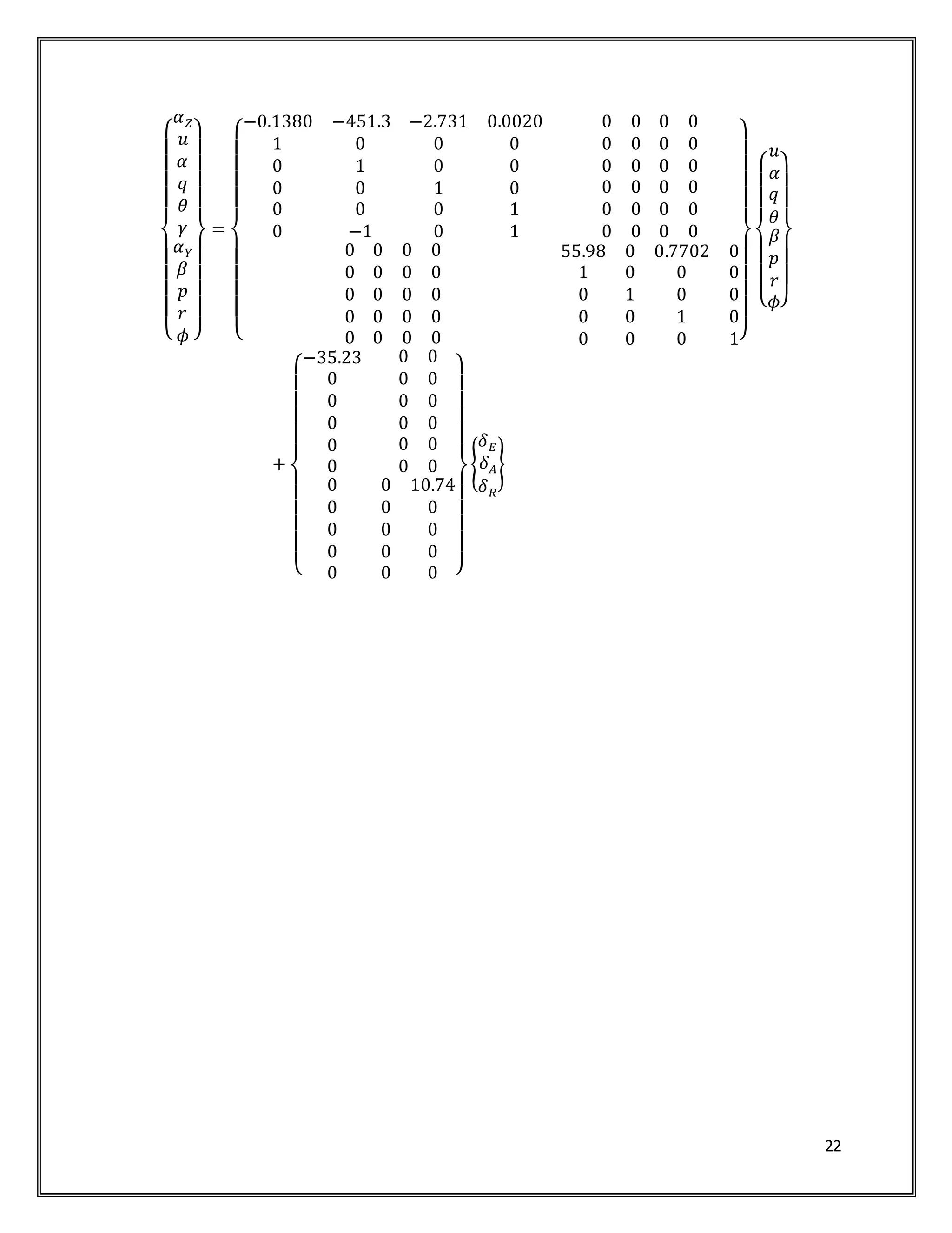
This changes the output equation for the aircraft as shown below.
{
𝛼 𝑧
𝑢
𝛼
𝑞
𝜃 }
=
[
−0.1380 −451.3 −2.731 0.0020
1 0 0 0
0 1 0 0
0 0 1 0
0 0 0 1 ]
{
𝑢
𝛼
𝑞
𝜃
} +
[
−35.23
0
0
0
0 ]
{ 𝛿 𝐸}

19. 19
This describes the vertical acceleration augmentation to the output equation. Similarly,
the output equation can then be altered to include the flight path angle. This is done by changing
the output matrix as such.
{
𝛼 𝑧
𝑢
𝛼
𝑞
𝜃
𝛾 }
=
[
−0.1380 −451.3 −2.731 0.0020
1 0 0 0
0 1 0 0
0 0 1 0
0 0 0 1
0 −1 0 1 ]
{
𝑢
𝛼
𝑞
𝜃
} +
[
−35.23
0
0
0
0
0 ]
{ 𝛿 𝐸}
3.2 Lateral State Variable Model
When solving the state variable model for the lateral direction, a set of steps is carried
out. First, the dimensional derivatives for the aircraft must be known. These derivatives are
from the aircraft dynamics and are shown in the table below.
Table 4: Lateral Stability and Control Derivatives
Lateral Stability and Control Derivatives
𝑌𝛽 55.98 𝐿 𝛽 -4.147 𝑁𝛽 2.839
𝑌𝑝 0 𝐿 𝑝 -0.4260 𝑁 𝑇𝛽
0
𝑌𝑟 0.7702 𝐿 𝑟 0.1515 𝑁 𝑝 -0.0045
𝑌𝛿 𝐴
0 𝐿 𝛿 𝐴
6.711 𝑁𝑟 -0.1123
𝑌𝛿 𝑅
10.74 𝐿 𝛿 𝑅
0.7163 𝑁𝛿 𝐴
-0.4471
𝑁𝛿 𝑟
-1.654
After these values are found, the single primed derivatives for the state variable model
are needed. These values are defined as follows.
Table 5: Lateral Single Primed Derivatives
Lateral Single Primed Derivatives
𝑌𝛽
′
0.0827 𝐿 𝛽
′
-4.107 𝑁𝛽
′
2.804
𝑌𝑝
′
0 𝐿 𝑝
′
-0.4261 𝑁 𝑝
′
-0.0081
𝑌𝑟
′
-0.9989 𝐿 𝑟
′
0.1499 𝑁𝑟
′
-0.1110
𝑌𝜙
′
0.0475 𝐿 𝛿 𝐴
′
6.705 𝑁𝛿 𝐴
′
-0.3901
𝑌𝛿 𝐴
′
0 𝐿 𝛿 𝑅
′
0.6927 𝑁𝛿 𝑅
′
-1.649
𝑌𝛿 𝑅
′
0.0159

20. 20
The state equation for aircraft is generated from these derivatives. The state equation is
shown in the next formula.
{
𝛽̇
𝑝̇
𝑟̇
𝜙̇}
= [
0.0827 0 −0.9989 0.0475
−4.107 −0.4261 0.1499 0
2.804 −0.0081 −0.1110 0
0 1 0.0472 0
]{
𝛽
𝑝
𝑟
𝜙
} + [
0 0.0159
6.705 0.6927
−0.3901 −1.649
0 0
]{
𝛿 𝐴
𝛿 𝑅
}
Once the state equation is found, the output equation must be known. The first step in
solving for the output matrix is augmenting the matrix to include lateral acceleration. The first
step in including this in the output equation is solving for the double primed derivatives for the
aircraft. These values are shown in the following table.
Table 6: Lateral Double Primed Derivatives
Lateral Double Primed Derivatives
𝑌𝛽
′′
55.98 𝑌𝜙
′′
0
𝑌𝑝
′′
0 𝑌𝛿 𝐴
′′
0
𝑌𝑟
′′
0.7702 𝑌𝛿 𝑅
′′
10.74
These derivatives are added to the output equation for the system. The changes to the
output equation are expressed as follows.
{
𝛼 𝑌
𝛽
𝑝
𝑟
𝜙 }
=
[
55.98 0 0.7702 0
1 0 0 0
0 1 0 0
0 0 1 0
0 0 0 1]
{
𝛽
𝑝
𝑟
𝜙
} +
[
0 10.74
0 0
0 0
0 0
0 0 ]
{
𝛿 𝐴
𝛿 𝑅
}
3.3 Overall State Variable Model
The overall state variable model for the aircraft can be seen in the following equations
{
𝑢̇
𝛼̇
𝑞̇
𝜃̇
𝛽̇
𝑝̇
𝑟̇
𝜙̇ }
= {
𝐴 𝐿𝑜𝑛𝑔 0
0 𝐴 𝐿𝑎𝑡
}
{
𝑢
𝛼
𝑞
𝜃
𝛽
𝑝
𝑟
𝜙}
+ {
𝐵 𝐿𝑜𝑛𝑔 0
0 𝐵 𝐿𝑎𝑡
} {
𝛿 𝐸
𝛿 𝐴
𝛿 𝑅
}

21. 21
{
𝛼 𝑍
𝑢
𝛼
𝑞
𝜃
𝛾
𝛼 𝑌
𝛽
𝑝
𝑟
𝜙 }
= {
𝐶 𝐿𝑜𝑛𝑔 0
0 𝐶 𝐿𝑎𝑡
}
{
𝑢
𝛼
𝑞
𝜃
𝛽
𝑝
𝑟
𝜙}
+ {
𝐷 𝐿𝑜𝑛𝑔 0
0 𝐷 𝐿𝑎𝑡
}{
𝛿 𝐸
𝛿 𝐴
𝛿 𝑅
}
Where:
{
𝑢̇
𝛼̇
𝑞̇
𝜃̇
𝛽̇
𝑝̇
𝑟̇
𝜙̇}
=
{
−0.0197 8.435 0 −32.16
0 −0.6644 0.9960 −0.0022
0 −7.112 −1.321 0
0 0 1 0
0 0 0 0
0 0 0 0
0 0 0 0
0 0 0 0
0 0 0 0
0 0 0 0
0 0 0 0
0 0 0 0
0.0827 0 −0.9989 0.0475
−4.107 −0.4261 0.1499 0
2.804 −0.0081 −0.1110 0
0 1 0.0472 0 }
+
{
0
−0.0520
−14.27
0
0 0
0 0
0 0
0 0
0
0
0
0
0 0.0159
6.705 0.6927
−0.3901 −1.649
0 0 }
{
𝛿 𝐸
𝛿 𝐴
𝛿 𝑅
}

22. 22
{
𝛼 𝑍
𝑢
𝛼
𝑞
𝜃
𝛾
𝛼 𝑌
𝛽
𝑝
𝑟
𝜙 }
=
{
−0.1380 −451.3 −2.731 0.0020
1 0 0 0
0 1 0 0
0 0 1 0
0 0 0 1
0 −1 0 1
0 0 0 0
0 0 0 0
0 0 0 0
0 0 0 0
0 0 0 0
0 0 0 0
0 0 0 0
0 0 0 0
0 0 0 0
0 0 0 0
0 0 0 0
55.98 0 0.7702 0
1 0 0 0
0 1 0 0
0 0 1 0
0 0 0 1}
{
𝑢
𝛼
𝑞
𝜃
𝛽
𝑝
𝑟
𝜙}
+
{
−35.23
0
0
0
0
0
0 0
0 0
0 0
0 0
0 0
0 0
0
0
0
0
0
0 10.74
0 0
0 0
0 0
0 0 }
{
𝛿 𝐸
𝛿 𝐴
𝛿 𝑅
}

23. 23
4 Simulation Results
4.1 Longitudinal Direction
Once the state variable matrix is fully defined for the aircraft, it is possible to simulate the
results. First, the results for the longitudinal direction are found. These are shown in the figure
below.
Figure 2: Longitudinal Simulation Results for Elevator Deflection
These graphs show the result of the system when a generic elevator maneuver is applied
to the aircraft. Along with the system response, one other comparison must be made. The
eigenvalues of the state matrix must match the roots of the characteristic equation for the aircraft.
This comparison is shown below.
0 50 100 150
-5
0
5
Time (s)
a(z)(g)
0 50 100 150
-10
0
10
Time (s)
a(g)0 50 100 150
-10
0
10
Time (s)
u(ft/s)
0 50 100 150
-20
0
20
Time (s)
q(deg)
0 50 100 150
-10
0
10
Time (s)
theta(deg)
0 50 100 150
-5
0
5
Time (s)
gamma(deg)
0 50 100 150
-5
0
5
Time (s)
dE(deg)

24. 24
Figure 3: Comparison of the Roots and Eigenvalues of the Aircraft
This figure shows how the eigenvalues of the state matrix match the pole location of the
characteristic equation for the aircraft.
4.2 Lateral Direction
Following the longitudinal direction, it is possible to simulate the lateral direction. The
first case taken into account is for a basic aileron doublet. This response is shown below.
-1.4 -1.2 -1 -0.8 -0.6 -0.4 -0.2 0
-4
-2
0
2
4
Longitudinal Pole Locations
Real Axis
ImaginaryAxis
-1.4 -1.2 -1 -0.8 -0.6 -0.4 -0.2 0
-4
-2
0
2
4
Eigenvalues of State Matrix
Real Axis
ImaginaryAxis

25. 25
Figure 4: Lateral Simulation Results for Aileron Deflection
Along with the response for an aileron deflection, the system can be simulated for a
rudder deflection. The results of the simulation for a rudder deflection are shown in the next
figure.
0 20 40 60
-0.2
0
0.2
Time (s)
a(y)(g)
0 20 40 60
-5
0
5
Time (s)
b(g)
0 20 40 60
-20
0
20
Time (s)
p(ft/s)
0 20 40 60
-10
0
10
Time (s)
r(deg)
0 20 40 60
-50
0
50
Time (s)
phi(deg)
0 20 40 60
-5
0
5
Time (s)
da(deg)

26. 26
Figure 5 Lateral Simulation Results for Rudder Deflection
These graphs show how both the dutch roll and spiral modes are unstable. To verify this
result, the eigenvalues of the state matrix are compared to the roots of the characteristic equation
for the aircraft. This comparison is made in the next figure
0 20 40 60
-0.2
0
0.2
Time (s)
a(y)(g)
0 20 40 60
-5
0
5
Time (s)
b(g)
0 20 40 60
-20
0
20
Time (s)
p(ft/s)
0 20 40 60
-10
0
10
Time (s)
r(deg)
0 20 40 60
-10
0
10
Time (s)
phi(deg)
0 20 40 60
-1
0
1
Time (s)
da(deg)

27. 27
Figure 6: Comparison of the Roots and Eigenvalues of the Aircraft
These figures are identical and show how the aircraft has an unstable dutch roll, along
with, an unstable spiral mode.
-0.6 -0.5 -0.4 -0.3 -0.2 -0.1 0 0.1
-2
-1
0
1
2
Lateral Pole Locations
Real Axis
ImaginaryAxis
-0.5 -0.4 -0.3 -0.2 -0.1 0 0.1
-2
-1
0
1
2
Eigenvalues of State Matrix
Real Axis
ImaginaryAxis

28. 28
5 Sensitivity Analysis
5.1 Variations of 𝒄 𝑳 𝜶
To begin the sensitivity analysis, the design value for the aircraft is found. This value is
listed below.
Variation of 𝑐 𝐿 𝛼
base value 5.84
This value is then varied from positive to negative twenty percent. When this is done the
following figures can be generated.
Figure 7: Sensitivity Analysis for 𝒄 𝑳 𝜶
2.77
2.78
2.79
2.8
2.81
2.82
2.83
2.84
2.85
4.672
4.9056
5.1392
5.3728
5.6064
5.84
6.0736
6.3072
6.5408
6.7744
7.008
ωnsp
CLα
Short Period ωn vs. CLα
0.31
0.32
0.33
0.34
0.35
0.36
0.37
0.38
4.672
4.9056
5.1392
5.3728
5.6064
5.84
6.0736
6.3072
6.5408
6.7744
7.008
dsp
CLa
Short Period ζ vs. CLα
0.087
0.088
0.089
0.09
0.091
0.092
0.093
0.094
4.672
4.9056
5.1392
5.3728
5.6064
5.84
6.0736
6.3072
6.5408
6.7744
7.008
omph
CLa
Phugoid ωn vs. CLα
0.095
0.096
0.097
0.098
0.099
0.1
0.101
0.102
0.103
0.104
0.105
0.106
dph
CLa
Phugoid ζ vs. CLα

29. 29
5.2 Variations of 𝒄 𝒎 𝜶
To begin the sensitivity analysis, the design value for the aircraft is found. This value is
listed below.
Variation of 𝑐 𝑚 𝛼
base value -0.64
This value is then varied from positive to negative twenty percent. When this is done the
following figures can be generated.
Figure 8: Sensitivity Analysis for 𝒄 𝒎 𝜶
5.3 Variations of 𝒄𝒍 𝜷
To begin the sensitivity analysis, the design value for the aircraft is found. This value is
listed below.
Variation of 𝑐𝑙 𝛽
base value -0.11
This value is then varied from positive to negative twenty percent. When this is done the
following figures can be generated.
0
0.5
1
1.5
2
2.5
3
3.5
omsp
Cma
Short Period ωn vs. Cmα
0
0.05
0.1
0.15
0.2
0.25
0.3
0.35
0.4
0.45
-0.512
-0.5376
-0.5632
-0.5888
-0.6144
-0.64
-0.6656
-0.6912
-0.7168
-0.7424
-0.768
dsp
Cma
Short Period ζ vs. Cmα

30. 30
Figure 9: Sensitivity Analysis for 𝒄𝒍 𝜷
5.4 Variations of 𝒄 𝒏 𝜷
To begin the sensitivity analysis, the design value for the aircraft is found. This value is
listed below.
Variation of 𝑐 𝑛 𝛽
base value 0.127
This value is then varied from positive to negative twenty percent. When this is done the
following figures can be generated.
1.68165
1.6817
1.68175
1.6818
1.68185
-0.088
-0.0924
-0.0968
-0.1012
-0.1056
-0.11
-0.1144
-0.1188
-0.1232
-0.1276
-0.132
omdr
Clb
Dutch Roll ωn vs. Clβ
0
0.005
0.01
0.015
0.02
-0.088
-0.0924
-0.0968
-0.1012
-0.1056
-0.11
-0.1144
-0.1188
-0.1232
-0.1276
-0.132
ddr
Clb
Dutch Roll ζ vs. Clβ
1.9
1.92
1.94
1.96
1.98
2
2.02
2.04
2.06
-0.088
-0.0924
-0.0968
-0.1012
-0.1056
-0.11
-0.1144
-0.1188
-0.1232
-0.1276
-0.132
troll
Clb
RollTime vs. Clβ
-10000
-8000
-6000
-4000
-2000
0
2000
4000
6000
8000
-0.088
-0.0924
-0.0968
-0.1012
-0.1056
-0.11
-0.1144
-0.1188
-0.1232
-0.1276
-0.132
tspr
Clb
Sprial Time vs. Clβ

31. 31
Figure 10: Sensitivity Analysis for 𝒄 𝒏 𝜷
5.5 Variations of 𝒄 𝒎 𝒖
To begin the sensitivity analysis, the design value for the aircraft is found. This value is
listed below.
Variation of 𝑐 𝑚 𝑢
base value 0.05
This value is then varied from positive to negative twenty percent. When this is done the
following figures can be generated.
0
0.5
1
1.5
2
omdr
Cnb
Dutch Roll ωn vs. Cnβ
0
0.005
0.01
0.015
0.02
0.025
0.1016
0.10668
0.11176
0.11684
0.12192
0.127
0.13208
0.13716
0.14224
0.14732
0.1524
ddr
Cnb
Dutch Roll ζ vs. Cnβ
1.85
1.9
1.95
2
2.05
2.1
0.1016
0.10668
0.11176
0.11684
0.12192
0.127
0.13208
0.13716
0.14224
0.14732
0.1524
troll
Cnb
RollTime vs. Cnβ
-15000
-10000
-5000
0
5000
0.1016
0.10668
0.11176
0.11684
0.12192
0.127
0.13208
0.13716
0.14224
0.14732
0.1524
tspr
Cnb
Sprial Time vs. Cnβ

32. 32
Figure 11: Sensitivity Analysis for 𝒄 𝒎 𝒖
5.6 Variations of 𝒄 𝒎 𝒒
To begin the sensitivity analysis, the design value for the aircraft is found. This value is
listed below.
Variation of 𝑐 𝑚 𝑞
base value -15.5
This value is then varied from positive to negative twenty percent. When this is done the
following figures can be generated.
Figure 12: Sensitivity Analysis for 𝒄 𝒎 𝒒
0.086
0.087
0.088
0.089
0.09
0.091
0.092
0.093
0.094
0.095
0.04
0.042
0.044
0.046
0.048
0.05
0.052
0.054
0.056
0.058
0.06
omph
Cmu
Phugoid ωn vs. Cmu
0.1005
0.101
0.1015
0.102
0.1025
0.103
0.04
0.042
0.044
0.046
0.048
0.05
0.052
0.054
0.056
0.058
0.06
dph
Cmu
Phugoid ζ vs. Cmu
2.77
2.78
2.79
2.8
2.81
2.82
2.83
2.84
2.85
omsp
Cmq
Short Period ωn vs. Cmq
0.29
0.3
0.31
0.32
0.33
0.34
0.35
0.36
0.37
0.38
0.39
dsp
Cmq
Short Period ζ vs. Cmq

33. 33
5.7 Variations of 𝒄𝒍 𝒑
To begin the sensitivity analysis, the design value for the aircraft is found. This value is
listed below.
Variation of 𝑐𝑙 𝑝
base value -0.45
This value is then varied from positive to negative twenty percent. When this is done the
following figures can be generated.
Figure 13: Sensitivity Analysis for 𝒄𝒍 𝒑
5.8 Variations of 𝒄 𝒏 𝒓
To begin the sensitivity analysis, the design value for the aircraft is found. This value is
listed below.
Variation of 𝑐 𝑛 𝑟
base value -0.2
This value is then varied from positive to negative twenty percent. When this is done the
following figures can be generated.
0
0.5
1
1.5
2
2.5
3
-0.36
-0.369
-0.378
-0.387
-0.396
-0.405
-0.414
-0.423
-0.432
-0.441
-0.45
-0.459
-0.468
-0.477
-0.486
-0.495
-0.504
-0.513
-0.522
-0.531
-0.54
troll
Clp
RollTime vs. Clp

34. 34
Figure 14: Sensitivity Analysis for 𝒄 𝒏 𝒓
1.6785
1.679
1.6795
1.68
1.6805
1.681
1.6815
1.682
1.6825
1.683
1.6835
-0.16
-0.168
-0.176
-0.184
-0.192
-0.2
-0.208
-0.216
-0.224
-0.232
-0.24
omdr
Cnr
Dutch Roll ωn vs. Cnr
0
0.005
0.01
0.015
0.02
0.025
-0.16
-0.168
-0.176
-0.184
-0.192
-0.2
-0.208
-0.216
-0.224
-0.232
-0.24
ddr
Cnr
Dutch Roll ζ vs. Cnr
1.975
1.98
1.985
1.99
1.995
2
2.005
2.01
2.015
-0.16
-0.168
-0.176
-0.184
-0.192
-0.2
-0.208
-0.216
-0.224
-0.232
-0.24
troll
Cnr
RollTime vs. Cnr
-10000
-8000
-6000
-4000
-2000
0
2000
4000
6000
-0.16
-0.168
-0.176
-0.184
-0.192
-0.2
-0.208
-0.216
-0.224
-0.232
-0.24
tspr
Cnr
Sprial Time vs. Cnr

35. 35
6 Conclusions
Several conclusions can be drawn from the simulation results for the Learjet 24. First,
the aircraft has a stable short period and phugoid response. Although, it does not have a stable
dutch roll or spiral model. A more complex controller is necessary to control the lateral direction
of the aircraft. This model is far superior to the transfer function based model. Also, it will
allow for a more powerful control in the future.

36. 36
7.1 Reference
Marcello Napolitano

37. 37
8.1 Appendix A – Simple Matlab Code for Longitudinal Direction
%Aircraft:Cessna Learjet 24
%Flight Condition:Cruise (max weight)
%Reference Geometry
S=230;
cbar=7;
b=34;
xcgbar=0.32;
%Flight Condition Data
Vp1=677;
M=0.7;
alpha1=2.7/57.3;
theta1=alpha1;
q1=134.6;
g=32.2;
%Mass and Inertial Data
W=13000;
m=(W/g);
IxxB=28000;
IyyB=18800;
IzzB=47000;
IxzB=1300;
%Steady State Coefficients
CL1=0.41;
CD1=0.0335;
CTx1=0.0335;
Cm1=0;
CmT1=0;
%Longitudinal Stability Derivatives
CD0=0.0216;
CDu=0.104;
CDa=0.3;
CTxu=-0.07;
CL0=0.13;
CLu=0.4;
CLa=5.84;
CLadot=2.2;
CLq=4.7;
Cm0=0.05;
Cmu=0.05;
Cma=-0.64;
Cmadot=-6.7;
Cmq=-18.6;
CmTu=-0.003;
CmTa=0;
%Longitudinal Control Derivatives
CDdE=0;
CLdE=0.46;
CmdE=-1.24;

38. 38
%Longitudinal Dimensional Stability Derivatives
Xu=(-q1*S*(CDu+(2*CD1)))/(m*Vp1);
XTu=(q1*S*(CTxu+(2*(CTx1))))/(m*Vp1);
Xa=(-q1*S*(CDa-CL1))/(m);
Zu=(-q1*S*(CLu+(2*CL1)))/(m*Vp1);
Za=(-q1*S*(CLa+CD1))/m;
Zadot=-(q1*S*cbar*CLadot)/(2*m*Vp1);
Zq=-(q1*S*cbar*CLq)/(2*m*Vp1);
Mu=(q1*S*cbar*(Cmu+(2*Cm1)))/(IyyB*Vp1);
MTu=(q1*S*cbar*(CmTu+(2*CmT1)))/(IyyB*Vp1);
Ma=(q1*S*cbar*Cma)/IyyB;
MTa=(q1*S*cbar*CmTa)/IyyB;
Madot=(q1*S*cbar^2*Cmadot)/(2*IyyB*Vp1);
Mq=(q1*S*cbar^2*Cmq)/(2*IyyB*Vp1);
%Longitudinal Dimensional Control Derivatives
XdE=-(q1*S*CDdE)/m;
ZdE=-(q1*S*CLdE)/m;
MdE=(q1*S*cbar*CmdE)/IyyB;
%Primed Longitudinal Dimensional Stability Derivatives
XuP=(Xu+XTu);
XaP=Xa;
XthetaP=-g*cos(theta1);
XqP=0;
XdEP=XdE;
ZuP=Zu/(Vp1-Zadot);
ZaP=Za/(Vp1-Zadot);
ZqP=(Zq+Vp1)/(Vp1-Zadot);
ZthetaP=-(g*sin(theta1))/(Vp1-Zadot);
ZdEP=ZdE/(Vp1-Zadot);
MuP=(Madot*ZuP)+Mu;
MaP=(Madot*ZaP)+Ma;
MthetaP=Madot*ZthetaP;
MqP=(Madot*ZqP)+Mq;
MdEP=(Madot*ZdEP)+MdE;
%Double Primed Longitudinal Dimensional Stability Derivatives
ZuPP=ZuP*Vp1;
ZaPP=(ZaP*Vp1)-(g*sin(theta1));
ZqPP=(ZqP-1)*Vp1;
ZthetaPP=(ZthetaP*Vp1)+(g*sin(theta1));
ZdEPP=ZdEP*Vp1;
%State Matricies
A=[XuP XaP XqP XthetaP
ZuP ZaP ZqP ZthetaP
MuP MaP MqP MthetaP
0 0 1 0];
B=[XdEP
ZdEP
MdEP
0];
C=[ZuPP ZaPP ZqPP ZthetaPP
1 0 0 0

39. 39
0 1 0 0
0 0 1 0
0 0 0 1
0 -1 0 1];
D=[ZdEPP
0
0
0
0
0];
sysSS=ss(A,B,C,D);
%Simulation
tSS=[0:.01 :120];
sizet=max(size(tSS));
for hi=1:sizet;
dESS(hi)=0;
end;
for hi=200:300;
dESS(hi)=-3/57.3;
end;
for hi=700:800;
dESS(hi)=3/57.3;
end;
y=lsim(sysSS,dESS,tSS);
azSS=y(:,1)*(1/32.17)+1;
aSS=y(:,3)*57.3;
uSS=y(:,2);
qSS=y(:,4)*57.3;
thetaSS=y(:,5)*57.3;
gamSS=y(:,6)*57.3
dESS=dESS*57.3;
%Plotting
clf;
hold on
grid on
d=eig(A);
figure(1)
plot(d,'k*')
omsp=sqrt(abs(d(1,1)^2))
dampsp=abs(real(d(1,1)))/(omsp)
omph=sqrt(abs(d(3,1)^2))
dampph=abs(real(d(3,1)))/(omph)
figure(2)
subplot(4,2,1);
plot(tSS,azSS,'k');
xlabel('Time (s)');
ylabel('a(z) (g)');
grid on
subplot(4,2,2);
plot(tSS,aSS,'k');
xlabel('Time (s)');

40. 40
ylabel('a (g)');
grid on
subplot(4,2,3);
plot(tSS,uSS,'k');
xlabel('Time (s)');
ylabel('u (ft/s)');
grid on
subplot(4,2,4);
plot(tSS,qSS,'k');
xlabel('Time (s)');
ylabel('q (deg)');
grid on
subplot(4,2,5);
plot(tSS,thetaSS,'k');
xlabel('Time (s)');
ylabel('theta (deg)');
grid on
subplot(4,2,6);
plot(tSS,gamSS,'k');
xlabel('Time (s)');
ylabel('gamma (deg)');
grid on
subplot(4,2,7);
plot(tSS,dESS,'k');
xlabel('Time (s)');
ylabel('dE (deg)');
grid on

41. 41
8.2 Appendix B – Simple Matlab Code for Lateral Direction
%Aircraft:Cessna Learjet 24
%Flight Condition:Cruise (max weight)
%Flight Condition
Vp1=677;
M=0.7;
alpha1=2.7/57.3;
theta1=alpha1;
q1=134.6;
g=32.2;
cbar=7;
b=34;
xcgbar=0.32;
S=230;
%Mass and Inertial Properties
W=13000;
m=(W/g);
IxxB=28000;
IyyB=18800;
IzzB=47000;
IxzB=1300;
%Lateral Directional Stability Derivatives
Clb=-0.11;
Clp=-0.45;
Clr=0.16;
Cyb=--0.73;
Cyp=0;
Cyr=0.4;
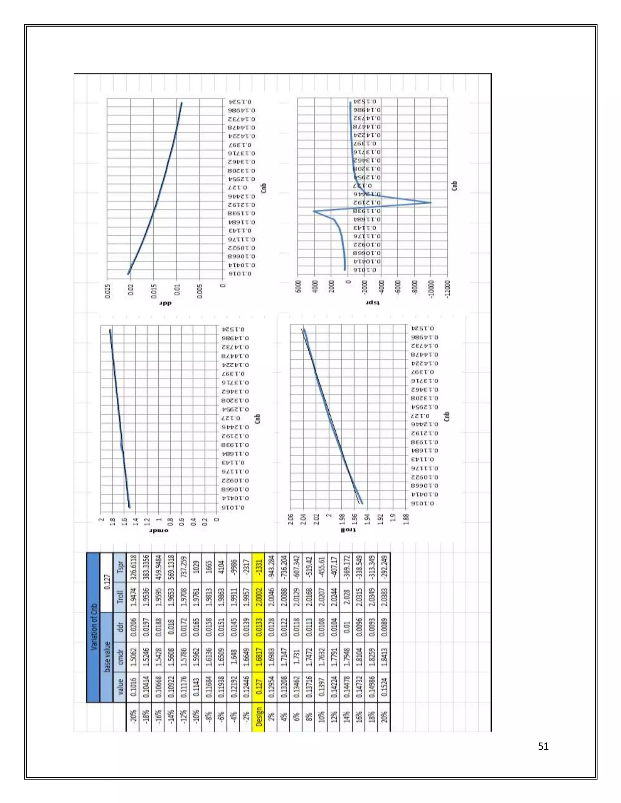
Cnb=0.127;
Cnp=-0.008;
Cnr=-0.24;
%Lateral Directional Control Derivatives
Clda=0.178;
Cldr=0.019;
Cyda=0;
Cydr=0.14;
Cnda=-0.02;
Cndr=-0.074;
%Matrix Transformation of the Moments of Inertia
A=[(cos(alpha1))^2,(sin(alpha1))^2,-sin(2*alpha1);
(sin(alpha1))^2,(cos(alpha1))^2,sin(2*alpha1);
(0.5*sin(2*alpha1)),(-0.5*sin(2*alpha1)),(cos(2*alpha1))];
moi=[IxxB IzzB IxzB]';
c=A*moi;
Ixx=c(1,1);
Izz=c(2,1);
Ixz=c(3,1);
I1=(Ixz/Ixx);
I2=(Ixz/Izz);

42. 42
%Lateral Directional Dimensional Stability Derivatives
Yb=(q1*S*Cyb)/m;
Yp=(q1*S*b*Cyp)/(2*m*Vp1);
Yr=(q1*S*b*Cyr)/(2*m*Vp1);
Lb=(q1*S*b*Clb)/Ixx;
Lp=(q1*S*(b^2)*Clp)/(2*Ixx*Vp1);
Lr=(q1*S*(b^2)*Clr)/(2*Ixx*Vp1);
Nb=(q1*S*b*Cnb)/Izz;
Np=(q1*S*(b^2)*Cnp)/(2*Izz*Vp1);
Nr=(q1*S*(b^2)*Cnr)/(2*Izz*Vp1);
%Lateral Directional Dimensional Control Derivatives
Yda=(q1*S*Cyda)/m;
Ydr=(q1*S*Cydr)/m;
Lda=(q1*S*b*Clda)/Ixx;
Ldr=(q1*S*b*Cldr)/Ixx;
Nda=(q1*S*b*Cnda)/Izz;
Ndr=(q1*S*b*Cndr)/Izz;
%Primed Lateral Dimensional Stability Derivatives
YbP=Yb/Vp1;
YpP=Yp/Vp1;
YrP=(Yr-Vp1)/Vp1;
YphiP=g*cos(theta1)/Vp1;
YdaP=Yda/Vp1;
YdrP=Ydr/Vp1;
LbP=(Lb+I1*Nb)/(1-I1*I2);
LpP=(Lp+I1*Np)/(1-I1*I2);
LrP=(Lr+I1*Nr)/(1-I1*I2);
LdaP=(Lda+I1*Nda)/(1-I1*I2);
LdrP=(Ldr+I1*Ndr)/(1-I1*I2);
NbP=(I2*Lb+Nb)/(1-I1*I2);
NpP=(I2*Lp+Np)/(1-I1*I2);
NrP=(I2*Lr+Nr)/(1-I1*I2);
NdaP=(I2*Lda+Nda)/(1-I1*I2);
NdrP=(I2*Ldr+Ndr)/(1-I1*I2);
%Double Primed Longitudinal Dimensional Stability Derivatives
YbPP=YbP*Vp1;
YpPP=YpP*Vp1;
YrPP=Vp1*(YrP+1);
YphiPP=(YphiP*Vp1)-(g*cos(theta1));
YdaPP=YdaP*Vp1;
YdrPP=YdrP*Vp1;
%State Matricies
A=[YbP YpP YrP YphiP
LbP LpP LrP 0
NbP NpP NrP 0
0 1 tan(theta1) 0];
B=[YdaP YdrP
LdaP LdrP
NdaP NdrP
0 0];
C=[YbPP YpPP YrPP YphiPP
1 0 0 0

43. 43
0 1 0 0
0 0 1 0
0 0 0 1];
D=[YdaPP YdrPP
0 0
0 0
0 0
0 0];
sysSS=ss(A,B,C,D);
d=eig(A)
omdr=sqrt(abs(d(2,1)^2))
ddr=(abs(real(d(2,1)))/omdr)
troll=-1/(d(3,1))
tspr=-1/(d(4,1))
%Simulation
tSS=[0:0.01:60];
sizet=max(size(tSS));
for hi=1:sizet;
dr(hi,1)=0;
da(hi,1)=0;
end;
for hi=200:300;
dr(hi,1)=-1/57.3;
end;
for hi=2200:2300;
dr(hi,1)=1/57.3;
end
u=[da,dr];
y=lsim(sysSS,u,tSS);
aySS=y(:,1)*(1/32.17);
pSS=y(:,3)*57.3;
bSS=y(:,2)*57.3;
rSS=y(:,4)*57.3;
phiSS=y(:,5)*57.3;
daSS=da*57.3;
drSS=dr*57.3;
%Plotting
clf;
hold on
figure(1)
subplot(3,2,1);
plot(tSS,aySS,'k');
xlabel('Time (s)');
ylabel('a(y) (g)');
grid on
subplot(3,2,2);

44. 44
plot(tSS,bSS,'k');
xlabel('Time (s)');
ylabel('b (g)');
grid on
subplot(3,2,3);
plot(tSS,pSS,'k');
xlabel('Time (s)');
ylabel('p (ft/s)');
grid on
subplot(3,2,4);
plot(tSS,rSS,'k');
xlabel('Time (s)');
ylabel('r (deg)');
grid on
subplot(3,2,5);
plot(tSS,phiSS,'k');
xlabel('Time (s)');
ylabel('phi (deg)');
grid on
subplot(3,2,6);
plot(tSS,drSS,'k');
xlabel('Time (s)');
ylabel('da (deg)');
grid on
figure(2);
plot(poles,'k*');
grid on
title('Lateral Pole Locations');
xlabel('Real Axis');
ylabel('Imaginary Axis');

45. 45
8.3 Appendix C – Simulink Block Diagram
2nd:Selectone-two-threecontrolsurfacemaneauversforElevator,Ailerons,
orRudderbymovingtheswtichestothedesiredposition
RudderInputs
AileronInputs
ElevatorInputs
Scopesof
AircraftOutputs
Outputscanbeplotted
inMATLABaswell
State-SpaceAircraftSimulation
1st:Run'State_Variable_Modeling_of_the_Aircraft_Dynamics_V2''
codetogeneratecontrolsurfaceinputsandaircraftsystem
atachosenflightcondition
1st:Run'State_Variable_Modeling_of_the_Aircraft_Dynamics_V2''
codetogeneratecontrolsurfaceinputsandaircraftsystem
atachosenflightcondition
3rd:double-clickscopestoviewresponsesoractivate
plottingatendofMATLABcodetoplotviaworkspace
u
theta
r
q
phi
p
beta
az
ay
alpha
sim_phi
sim_r
sim_p
sim_beta
sim_ay
sim_theta
sim_q
sim_u
sim_alpha
sim_az
Mux
deltae3s
deltae1s
deltar3s
deltar1s
deltar2s
deltaa3s
deltaa1s
deltaa2s
deltae2s
x'=Ax+Bu
y=Cx+Du
AircraftState-Space

46. 46
8.4 Appendix D –Longitudinal Excel Spreadsheet

47. 47

48. 48

49. 49

50. 50
8.5 Appendix E –Lateral Excel Spreadsheet

51. 51

52. 52

53. 53