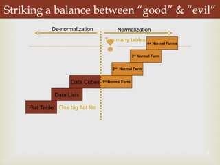
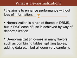
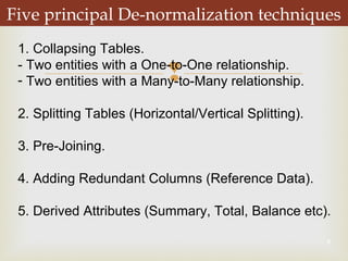
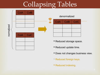
1
Lecture-7Lecture-7
De-normalizationDe-normalization
Mamuna Fatima

2
Striking a balance between “good” & “evil”
Flat Table
Data Lists
Data Cubes 1st
Normal Form
2nd
Normal Form
3rd
Normal Form
4+ Normal Forms
NormalizationDe-normalization
One big flat file
Too many tables

3
What is De-normalization?
the aim is to enhance performance without
loss of information.
 Normalization is a rule of thumb in DBMS,
but in DSS ease of use is achieved by way of
denormalization.
 De-normalization comes in many flavors,
such as combining tables, splitting tables,
adding data etc., but all done very carefully.

 Bringing “close” dispersed but related data items.
 Very early studies showed performance difference in orders of
magnitude for different number de-normalized tables and rows
per table.
 The level of de-normalization should be carefully considered.
4
Why De-normalization In DSS?

5
How De-normalization improves performance?
De-normalization specifically improves
performance by either:
 Reducing the number of tables and hence the
reliance on joins, which consequently speeds up
performance.
 Reducing the number of joins required during
query execution, or
 Reducing the number of rows to be retrieved from
the Primary Data Table.

6
4 Guidelines for De-normalization
1. Carefully do a cost-benefit analysis
(frequency of use, additional storage,
join time).
2. Do a data requirement and storage
analysis.
3. Weigh against the maintenance issue
of the redundant data (triggers used).
4. When in doubt, don’t denormalize.

7
Areas for Applying De-Normalization Techniques
 Dealing with the abundance of star schemas.
 Fast access of time series data for analysis.
 Fast aggregate (sum, average etc.) results and
complicated calculations.
 Multidimensional analysis (e.g. geography) in a complex
hierarchy.
 Dealing with few updates but many join queries.
De-normalization will ultimately affect the database size and
query performance.

8
Five principal De-normalization techniques
1. Collapsing Tables.
- Two entities with a One-to-One relationship.
- Two entities with a Many-to-Many relationship.
2. Splitting Tables (Horizontal/Vertical Splitting).
3. Pre-Joining.
4. Adding Redundant Columns (Reference Data).
5. Derived Attributes (Summary, Total, Balance etc).

9
Collapsing Tables
ColA ColB
ColA ColC
normalized
ColA ColB ColC
denormalized
 Reduced storage space.
 Reduced update time.
 Does not changes business view.
 Reduced foreign keys.
 Reduced indexing.

9
Collapsing Tables
ColA ColB
ColA ColC
normalized
ColA ColB ColC
denormalized
 Reduced storage space.
 Reduced update time.
 Does not changes business view.
 Reduced foreign keys.
 Reduced indexing.

Dwh lecture-07-denormalization

  • 1.
  • 2.
     2 Striking a balancebetween “good” & “evil” Flat Table Data Lists Data Cubes 1st Normal Form 2nd Normal Form 3rd Normal Form 4+ Normal Forms NormalizationDe-normalization One big flat file Too many tables
  • 3.
     3 What is De-normalization? theaim is to enhance performance without loss of information.  Normalization is a rule of thumb in DBMS, but in DSS ease of use is achieved by way of denormalization.  De-normalization comes in many flavors, such as combining tables, splitting tables, adding data etc., but all done very carefully.
  • 4.
      Bringing “close”dispersed but related data items.  Very early studies showed performance difference in orders of magnitude for different number de-normalized tables and rows per table.  The level of de-normalization should be carefully considered. 4 Why De-normalization In DSS?
  • 5.
     5 How De-normalization improvesperformance? De-normalization specifically improves performance by either:  Reducing the number of tables and hence the reliance on joins, which consequently speeds up performance.  Reducing the number of joins required during query execution, or  Reducing the number of rows to be retrieved from the Primary Data Table.
  • 6.
     6 4 Guidelines forDe-normalization 1. Carefully do a cost-benefit analysis (frequency of use, additional storage, join time). 2. Do a data requirement and storage analysis. 3. Weigh against the maintenance issue of the redundant data (triggers used). 4. When in doubt, don’t denormalize.
  • 7.
     7 Areas for ApplyingDe-Normalization Techniques  Dealing with the abundance of star schemas.  Fast access of time series data for analysis.  Fast aggregate (sum, average etc.) results and complicated calculations.  Multidimensional analysis (e.g. geography) in a complex hierarchy.  Dealing with few updates but many join queries. De-normalization will ultimately affect the database size and query performance.
  • 8.
     8 Five principal De-normalizationtechniques 1. Collapsing Tables. - Two entities with a One-to-One relationship. - Two entities with a Many-to-Many relationship. 2. Splitting Tables (Horizontal/Vertical Splitting). 3. Pre-Joining. 4. Adding Redundant Columns (Reference Data). 5. Derived Attributes (Summary, Total, Balance etc).
  • 9.
     9 Collapsing Tables ColA ColB ColAColC normalized ColA ColB ColC denormalized  Reduced storage space.  Reduced update time.  Does not changes business view.  Reduced foreign keys.  Reduced indexing.
  • 10.
     9 Collapsing Tables ColA ColB ColAColC normalized ColA ColB ColC denormalized  Reduced storage space.  Reduced update time.  Does not changes business view.  Reduced foreign keys.  Reduced indexing.